6 Torsion
Moments can produce multiple effects on a body or structure, depending on the axes around which they act. Whereas later sections of the text discuss the effect of moments that cause bending are discussed (see Chapter 7, Chapter 9, Chapter 10, and Chapter 11), this chapter concerns the effects of moments that cause torsion.
Torsion occurs when a moment is applied around the longitudinal axis of a body. This type of moment is known as torque and the effect of torsion is a twisting action. Torsion is found in many common situations. Some examples of applications in which torsion is a primary form of loading include these:
In machinery, rotating shafts, such as transmission shafts that transmit power, are subjected to torque.
When one uses a wrench to tighten or loosen a bolt, the bolt is subjected to torque.
Hinge pins are subjected to torque when the rotating elements they are attached to (e.g., doors) are rotated.
Vertical poles from which road signs and traffic lights are mounted are subjected to torque when forces are applied to the horizontal elements of the structure. For example, in Figure 6.1 wind force applied to the horizontal poles or traffic lights causes the vertical pole to twist around the vertical axis.
Note that in this particular example the vertical pole would also be subject to bending (from moments around the cross-sectional axes of the pole). Problems in which this type of combined torsion and bending effects occur are discussed in Chapter 14.
This chapter focuses on the effects of pure torsion (no axial or bending loads) on bodies.
Section 6.1 describes the general effects of torsion. Section 6.2 details the process to determine internal torques as a preliminary step to stress and deformation calculations. Section 6.3 and Section 6.4 offer derivation equations for calculating the stress and deformation caused by torsional loads. Section 6.5 examines how these concepts can be applied to solving statically indeterminate torsion problems, which is a similar process as axial loading statically indeterminate problems described in Section 5.5. Finally, Section 6.6 considers how the concept of torque applies in power transmission applications.
6.1 The Effect of Torsion
Click to expand
As mentioned, a torsional moment causes the body to twist, and this action results in shear stress.
Consider the pleated tube shown in Figure 6.2. Figure 6.2 (A) shows the tube in an unloaded state with some of the pleats colored for identification. Figure 6.2 (B) shows that after a torque is applied, the pleats move vertically but not horizontally. We can say that all points remain in their original plane even as they twist to new locations around the perimeter of the cross-section. In other words, the shape of the cross-section is unchanged despite the twisting action.
.png)
Now consider the I-beam subjected to torsion in Figure 6.3. In this case the shape of the cross-section changes and the points do not remain in the same vertical plane (there is horizontal displacement as well as vertical). This shape change is referred to as warping. In this text we consider only circular cross-sections with no warping.
Returning to Figure 6.2, let’s consider the shape formed by the nondisplaced colored lines in Figure 6.2 (A) versus the displaced lines in Figure 6.2 (B). These images are shown again in Figure 6.4. In the nondisplaced case, a rectangle can be drawn around the green lines on the left with 90° corners. In the displaced case, the corners are no longer at 90°. From Section 3.4 we know that this change in angle is the definition of shear strain. The evidence of shear strain indicates that the applied torque results in shear stress.
6.2 Determination of Internal Torques
Click to expand
As with axial loading, stress and deformations from torsion vary from point to point within a body and are dependent on the internal torques at the individual points and on the geometric section properties. Internal torques can be found by sectioning bodies and applying equilibrium equations, just as we did when finding internal forces in axial loading problems (see Example 1.5, Example 2.1, and Example 2.2). In the case of internal torques, moment equilibrium around the longitudinal axis is applied instead of force summation.
Before we examine the process of finding internal torque reactions, it would be beneficial to establish the sign convention and ways of representing torque used in this text.
6.2.1 Sign Conventions and Representation of Torque
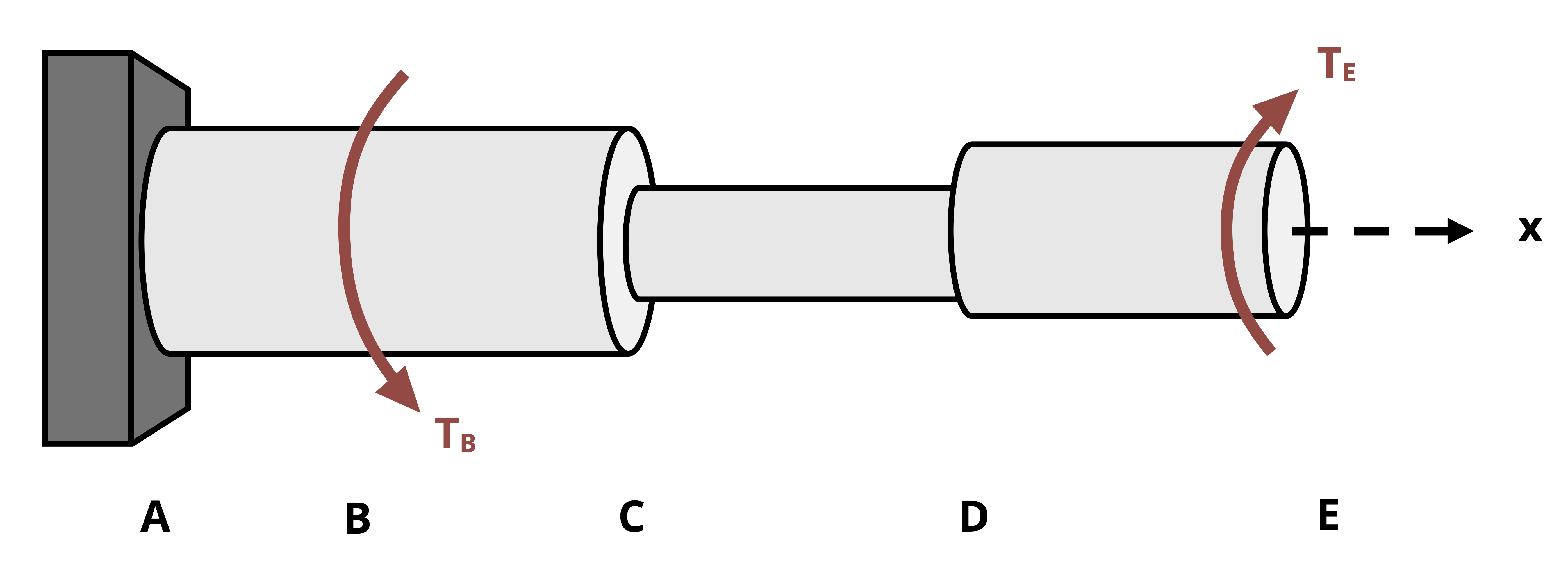
In this text counterclockwise torques are considered positive and clockwise torques negative. However, the apparent direction of a torque depends on the perspective from which the rotation is observed. In Figure 6.5, the applied torque would appear clockwise if viewed from the left end of the bar toward the right and counterclockwise if viewed from the right end of the bar toward the left. As long as you are consistent, which perspective is used isn’t usually important. However, a typical convention (and the one followed in this text) is to look from the free end of the shaft (if there is one) toward the fixed end, or from the positive end of the longitudinal toward the negative.
To visually determine whether a torque appears clockwise or counterclockwise can sometimes be difficult, so one helpful tool that can be used is the right-hand rule: Curl the fingers of your right hand in the direction of the rotation represented by the torque arrow. If in doing this your thumb points in the direction of the positive axis (the x-axis in Figure 6.6), a positive torque is indicated, and if it points away, a negative torque.
For bodies that are sectioned to find internal torques, consider the direction of the torsional moment from the perspective of looking from the cut edge towards the other end of the cut section. Imagine your right hand to be at the cut edge and curling your fingers in the direction of the torque. If your thumb points away from the cut edge, the internal torque is positive, and if your thumb points toward the cut edge, the internal torque is negative. This is illustrated in Figure 6.7.
Finally, since circular arrows can be difficult to draw in a way that clearly conveys direction, double-headed line arrows are frequently used to represent torque. Note that conventions can vary between texts and other sources. This text uses the following convention:
- On a whole body FBD used to determine external reactions, arrows facing in the direction of the positive longitudinal axis indicate positive torques (counterclockwise) and those facing the opposite direction negative torques.
- When applying equilibrium, the positive or negative sign from step 1 is used.
- For FBDs of cut sections used to determine internal torques, positive torques are indicated by arrows pointed away from the section’s cut edge, and negative torques by arrows pointed toward the cut edge. However, when summing moments, the regular convention of adding right arrows and subtracting left arrows will be used.
The direction of the internal torque is unimportant in calculating shear stress (the sign on the stress requires concepts discussed in Chapter 12) but is important when calculating angle of twist, as evident in Section 6.2.
Example 6.1 demonstrates how to determine internal torques in a multisection body as well as how to apply the described sign conventions.
Example 6.1
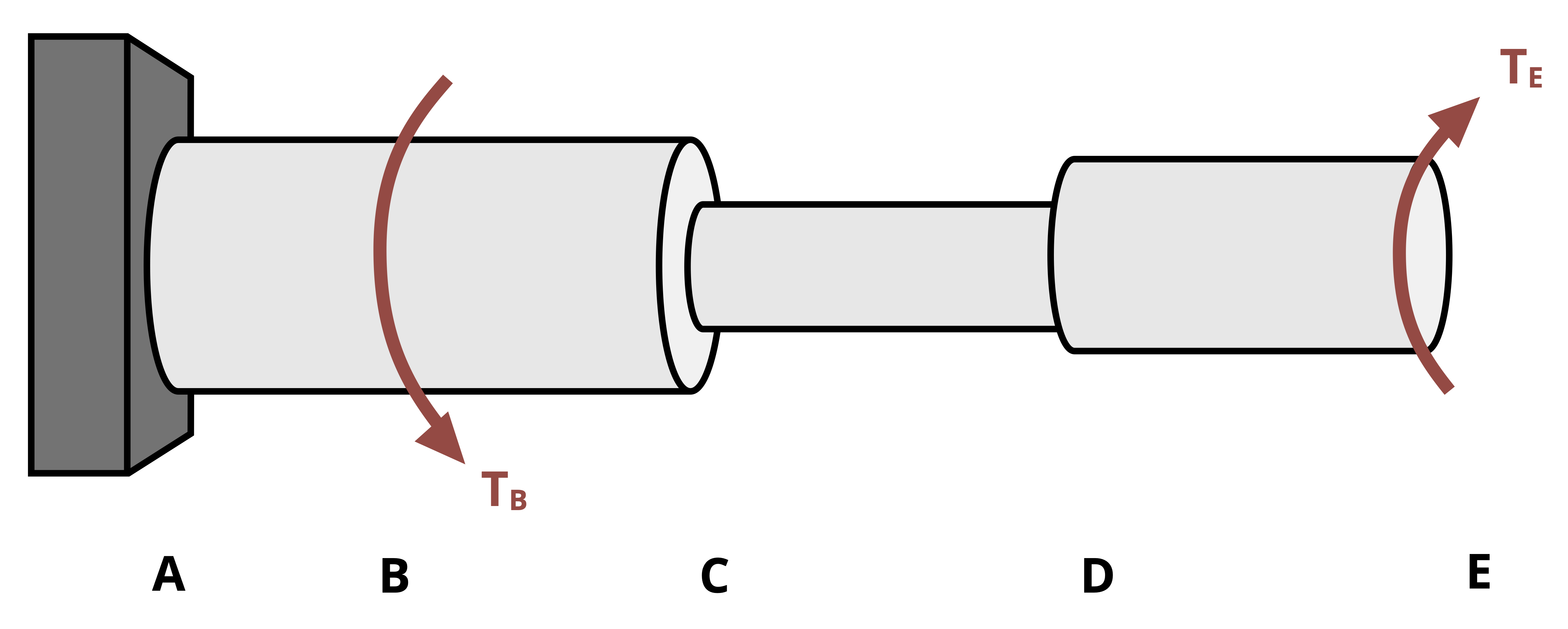
A multisection steel bar is supported by a fixed support at A and is subjected to torque TB = 70 N·mm and TE = 30 N·mm.
Determine the internal torque at all points in the shaft.
With torques applied only at points B and E (there is also a reaction moment from the wall at A), section AB and section BE are sections of constant internal torque. The reaction torque at A could be obtained by applying equilibrium to the whole shaft, but this example shows how to avoid that.
Section AB:
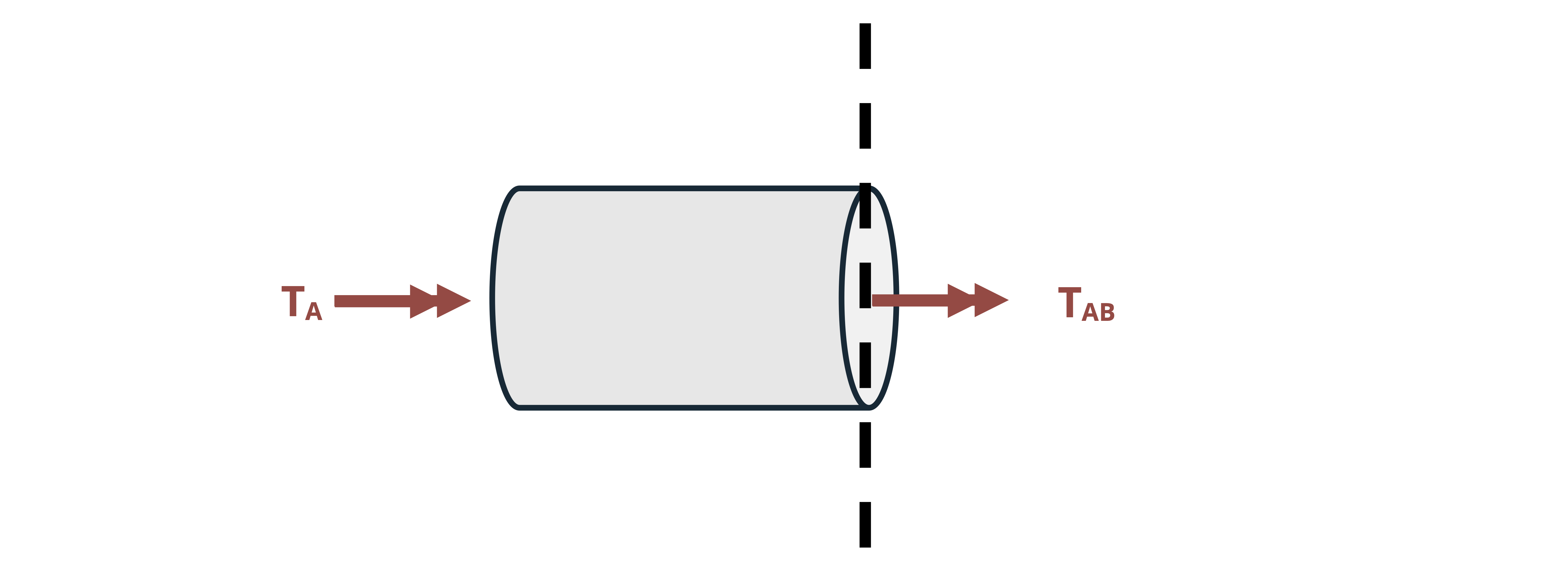
To determine the internal torque in section AB, we can cut the shaft anywhere between points A and B and draw an FBD of the section to the left of the cut or the section to the right of the cut.
Note that in the following illustration of the cut and the resulting FBDs, the internal torque TAB is drawn in opposite directions on the two sections. This must be the case if the bar is in equilibrium.
TAB is drawn as a positive internal torque on both the left and the right section diagrams since in both instances it points away from the cut. We assume that TAB looks counterclockwise if we view the left section from the cut toward A or the right section from the cut toward E.
For the applied loads, since TA is drawn in the direction opposite of TAB on the section to the left of the cut, it is assumed to appear clockwise from the cut toward A.
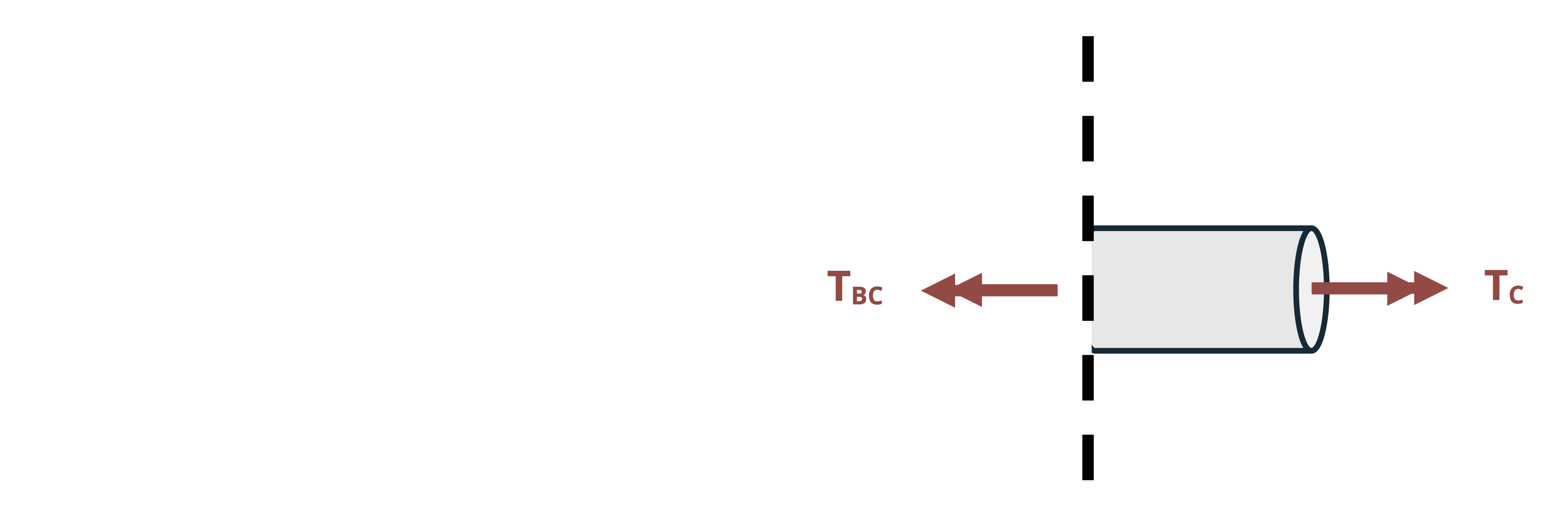
On the right side diagram, TB is drawn in the direction opposite of TAB since it appears clockwise from the cut toward E. Applied torque TE is drawn in the same direction as TAB since it appears counterclockwise from the cut toward E.
In writing the equilibrium equation to find TAB, we use either the left section FBD or the right section FBD and obtain the same result. To avoid needing to find TA, we will choose to use the right section FBD.
Recall that torques are moments around the longitudinal axis, which is the x-axis in this case. Applying the x-axis moment equilibrium equation to the right section gives
\[ \begin{aligned} \sum M_x&=-T_{AB}+T_B-T_E=0 \\ &=-T_{A B}+70{~N}\cdot{mm}-30{~N}\cdot{mm}=0 \\[10pt] T_{A B}&=40{~N}\cdot{mm}\ (counterclockwise) \end{aligned} \]
Note that in performing the summation, right directed arrows were added and vice versa. The opposite convention can also be used with the same end result.
The positive result for TAB in this case confirms that the assumed direction for TAB is the correct one, so it is a counterclockwise internal torque.
Section BE:
Similarly, the internal torque in all parts of the shaft between B and E can be determined by cutting the shaft at a nonspecific point between B and E and applying equilibrium to either the section of shaft to the left of the cut or the section to the right of the cut, as shown in the next two FBDs.
Once again the internal torque (TBE in this case) is drawn in the direction away from the cut on both sections, so it is assumed to be counterclockwise on both sections.
Applying the moment equilibrium equation on the right section results in
\[ \begin{aligned} \sum M_x&=-T_{BE}-T_E=0 \\ &=-T_{BE}-30{~}N\cdot{mm}=0 \\[10pt] T_{B E}&=-30{~N}\cdot{mm}\ (or\ 30{~} N\cdot{mm}\ clockwise) \end{aligned} \]
The negative result indicates that TBE goes in the opposite direction than what was assumed on the FBD, so it is clockwise.
Answer:
Internal torque for all points between A and B is 40 N·mm counterclockwise.
Internal torque for all points between B and E is 30 N·mm clockwise.
6.3 Calculation of Shear Stress Due to Pure Torsion
Click to expand
This section explains the derivation of the shear stress equation that results from torsion of a circular shaft. Understanding the derivation lends clarity to the inputs of the equation and the assumptions necessary for use. If you wish to skip the derivation, go directly to Equation 6.1.
Consider a circular shaft fixed on one end and subjected to torque on the free end, as shown in Figure 6.8. The shaft has an outer radius, c, as shown in Figure 6.9 (B). For the given loading, the internal torque at any x location along the length of the shaft would also be T. We will examine a small sliver of the shaft, marked as AB.
Before the torque is applied, a horizontal line segment drawn across AB has a length of Δx. Now let’s consider the same shaft segment after the torque has been applied and points A and B move to A’ and B’ respectively. We can approximate that A’B’ is linear for a very narrow section of shaft (infinitely small Δx). An illustration of the resulting geometry can be seen in Figure 6.9 (A). Since the shaft is fixed on the left end, point B on the shaft will rotate more than point A. Point A’’ represents the relative location of A’ on the cross-section of B and B’.
Recalling that shear strain is the change in angle between two lines that are originally perpendicular, we can see that the angle of tilt of A’B’ relative to the horizontal line A’A” is the shear strain, 𝛾, that results from the torque. For an infinitely small Δx, the arc segment from A” to B’ can be approximated as vertical so that the shear strain 𝛾 can be expressed using trigonometry.
\[ \tan (\gamma)=\frac{A^{\prime\prime} B^{\prime}}{\Delta x} \]
The small-angle approximation (given an infinitely small Δx) results in
\[ \tan(\gamma)\approx\gamma=\frac{A^{\prime\prime} B^{\prime}}{\Delta x} \]
Now consider the cross-section of the shaft where points B and B’ are located, shown in Figure 6.9 (B). The angle between the radial lines leading from the center to points A” and B’ respectively is the shaft segment’s angle of twist. Since we are examining a very small section of the shaft, the angle is represented as Δφ (as opposed to the absolute angle of twist, φ, as measured from the fixed end). If the shaft’s outer radius is r = c, then the length of A”B’ is given by the arc length, so
\[ \mathrm{A}^{\prime\prime}\mathrm{B}^{\prime}=\mathrm{c}(\Delta \phi) \]
and
\[ \gamma=\frac{c(\Delta \phi)}{\Delta x}\text{.} \]
Generalizing this result for any point on the cross-section that is located at an arbitrary radial distance ρ from the center yields
\[ \gamma=\frac{\rho(\Delta \phi)}{\Delta x}\text{.} \]
The resulting expression of γ shows that the shear strain varies linearly with ρ from the center of the cross-section to the outer radius, as illustrated in Figure 6.10. The shear strain is 0 at the center, and the maximum shear strain occurs at the max value of ρ which is ρ = c.
\[ \gamma_{\max }=\frac{c(\Delta \phi)}{\Delta x} \]
Substituting the general and max expressions for shear strain into Hooke’s law for shear stress, τ = G𝛾, reveals that shear stress also varies linearly from 0 to τmax in going from the center of the cross-section to the outer radius.
\[ \tau=G \gamma=G \frac{\rho(\Delta \phi)}{\Delta x}\\[10pt] \tau_{\max }=G \frac{c(\Delta \phi)}{\Delta x} \]
Figure 6.10 shows that the slope of the linear variation is \(\frac{\tau_{\max }}{c}\) and that the shear stress can also be expressed as
\[ \tau=\frac{\tau_{\max }}{c} \rho\text{.} \]
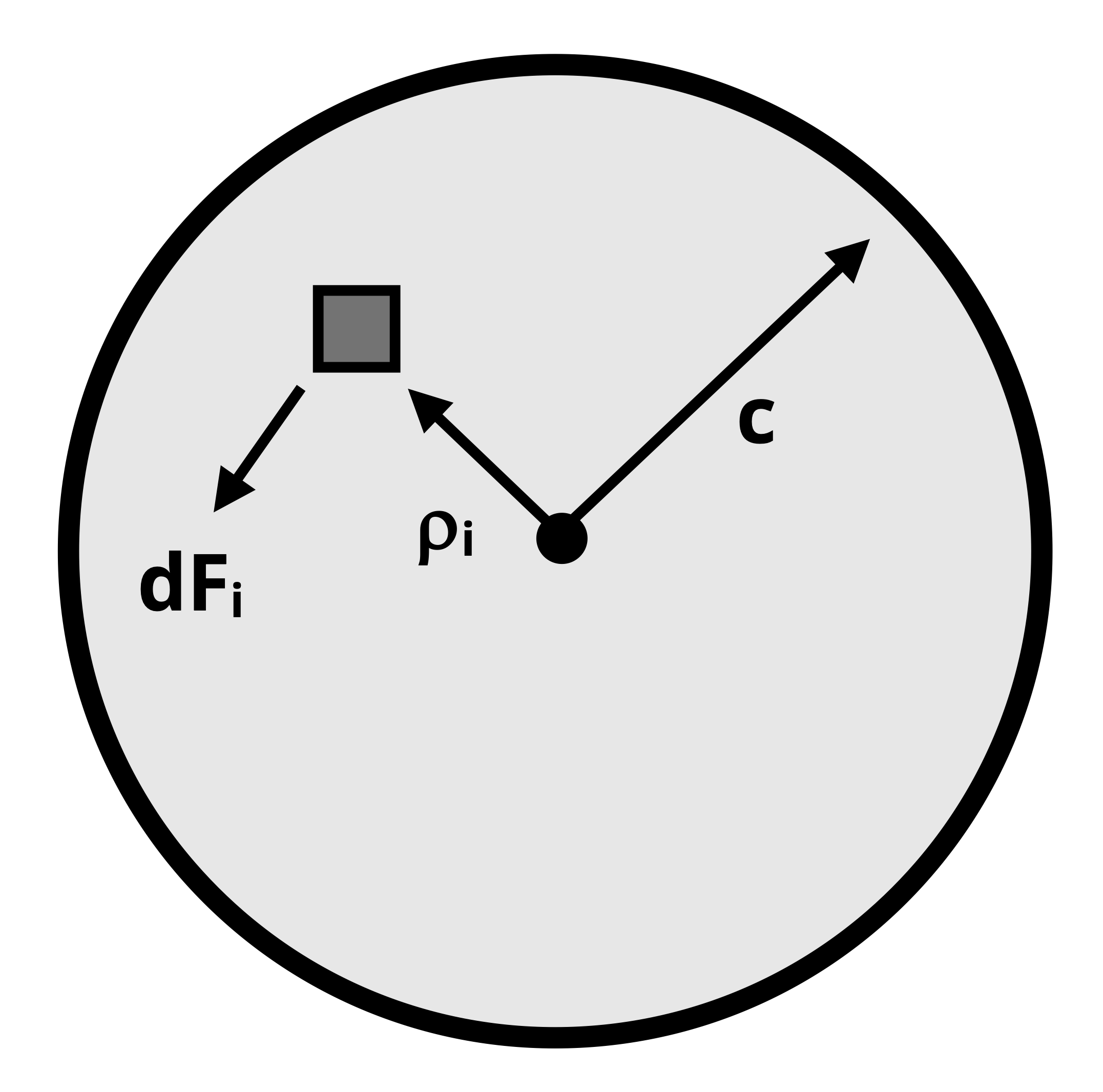
The last step in developing the shear stress relationship to torque involves considering the shaft’s equilibrium. Refer to Figure 6.11, in which the square is a representative point (i) subjected to an infinitesimal force dFi corresponding to the shear stress discussed above. If each point (i) on the cross-section has an area of dAi then dFi can be calculated as
\[ \mathrm{dF}_i=\tau_i \mathrm{dA}_i=\frac{\tau_{\max }}{c} \rho_i d A_i\text{.} \]
Recalling that the internal torque everywhere on the shaft is T, note that equilibrium dictates that the sum of the moments about the center of the cross-section should be equal to T. For an infinite number of points on the cross-section, this summation can be performed as an integral.
\[ \sum M_{center} =T=\int (d F_i) \ (\rho_i)=\int \frac{\tau_{\max }}{c} \rho_i^2 d A \]
Since τmax and c are constant, they can be pulled outside the integral, leaving the integral portion to be \(\int \rho_i^2 d A\), which is the definition of the polar second moment of area (also known as moment of inertia and area moment of inertia). This is the moment of inertia around the out-of-plane axis, which is the x-axis in this case. The polar second moment of area is denoted with the letter J in this text.
For a solid circular cross-section of outer radius r and outer diameter d:
\[ J_{solid}=\frac{\pi}{2} r^4=\frac{\pi}{32} d^4\text{.} \]
For a tube or hollow circular cross-section with outer radius and diameter ro and do respectively and inner radius and diameter ri and di respectively:
\[ J_{hollow}=\frac{\pi}{2}\left(r_o^4-r_i^4\right)=\frac{\pi}{32}\left(d_o^4-d_i^4\right)\text{.} \]
Replacing \(J=\int \rho^2_idA\) in our previous equation results in
\[ T=\frac{\tau_{\max } J}{c}\text{.} \]
This can be rearranged to
\[ \tau_{\max }=\frac{T c}{J}\text{.} \]
This equation yields the maximum stress on a given circular cross-section, which will occur on the outer edge of the shaft (where ρ = c). A more general form of the equation that can be used to find the stress at any point on the cross-section is
\[ \boxed{\tau=\frac{T \rho}{J}}\text{ ,} \tag{6.1}\]
𝜏 = Shear stress due to torsion [Pa, psi]
T = Internal torque [N·m, lb·in.]
𝜌 = Radial distance from center of cross-section to point of interest on the cross-section [m, in.]
J = Polar second moment of area [m4, in.4]
Here linear elastic behavior and small deformations of a circular cross-section have been assumed.
Note that for now only the magnitude of the shear stress (without sign) will be determined, since the sign for shear stress is not based purely on the sign of the torque. The sign on shear stress is discussed in Chapter 12.
Example 6.2 demonstrates the use of the above equations to determine shear stress in the same circular bar assembly used in Example 6.1.
Example 6.2
The multisection solid steel bar of Example 6.1 is repeated here with the same loading (TB = 70 N·mm and TE = 30 N·mm).
Also given the diameters dAC = 50 mm, dCD = 20 mm, and dDE = 35 mm, determine the magnitude and location of the maximum shear stress in the bar assembly.
6.4 Calculation of Angle of Twist
Click to expand
The deformation of a shaft that arises from applying torsion—assuming deformation is restricted to elastic deformation—is quantified by the angle of twist, φ. As discussed in Section 6.3 and illustrated here again in Figure 6.12, the angle of twist is the angle formed between the radial lines that correspond to the original location of a point on the cross-section and the location it moves to as a result of applied torque. The equation to determine angle of twist at various points along the shaft follows. If you wish to skip the derivation, go directly to Equation 6.2.
Recall from Section 6.3 that the shear strain can be expressed as \(\gamma=\frac{\rho(\Delta \phi)}{\Delta x}\). Also recall that Δx represents the length of a small section of shaft and Δφ is the change in angle of twist that occurs across that length. For an infinitely small section of shaft, the shear strain equation can be expressed in terms of differentials: \(\gamma=\frac{\rho(d \phi)}{d x}\).
Applying Hooke’s law (τ = G𝛾) and the equation for shear stress (Equation 6.1) yields
\[ \frac{\rho(d \phi)}{d x}=\frac{\tau}{G}=\frac{T \rho}{J G}\text{.} \]
Solving for dφ yields
\[ d \phi=\frac{T d x}{J G}\text{.} \]
Integrating both sides of the equation gives the total angle of twist for an entire shaft or section of shaft.
\[ \phi=\int \frac{T d x}{J G} \]
For a section (i) of shaft of length Li for which torque (Ti), material (Gi), and geometry (Ji), stay constant, this becomes
\[\phi_i=\frac{T_i L_i}{J_i G_i}\text{.} \]
For multisection bodies where each individual section has constant T, J, and G, the integral can be expressed in the form of a sum where the angle of twist of each distinct section is calculated individually and then all are added together.
\[ \boxed{\phi=\sum\phi_i=\sum \frac{T_i L_i}{J_i G_i}}\text{ ,} \tag{6.2}\]
𝜙 = Angle of twist [rad]
T = Internal torque [N·m, lb·in.]
L = Length [m, in.]
J = Polar moment of inertia [m4, in.4]
G = Shear modulus [Pa, psi]
In these calculations the sign of internal torque is important as it indicates the direction of the twist. If a section twists in one direction and the adjoining section twists in the opposite direction, the angles will subtract from each other, resulting in a smaller overall angle of twist. If, however, two adjoining sections twist in the same direction, the effect will be additive. According to the assumed sign convention discussed in Section 6.2, an overall positive angle of twist indicates that the shaft twists counterclockwise when looking from the positive end of the longitudinal axis to the negative and clockwise when looking from the negative to the positive end.
6.4.1 Units
If values for T, L, J, and G are used in Equation 6.2 such that the units are all consistent with each other, the overall unit works out to be unitless, as is expected for an angle calculation. Since the calculation is for an angle, the actual unit is in radians. To obtain an answer in degrees, convert the result of the equation by multiplying it by \(\frac{180^\circ}{\pi}\).
Because the angle of twist often works out to be very small, you may want to express the value in terms of μrad, which is 10-6 radians. To convert from rad to μrad, multiply the number of radians by 106.
6.4.2 Notation and Relative Angle of Twist
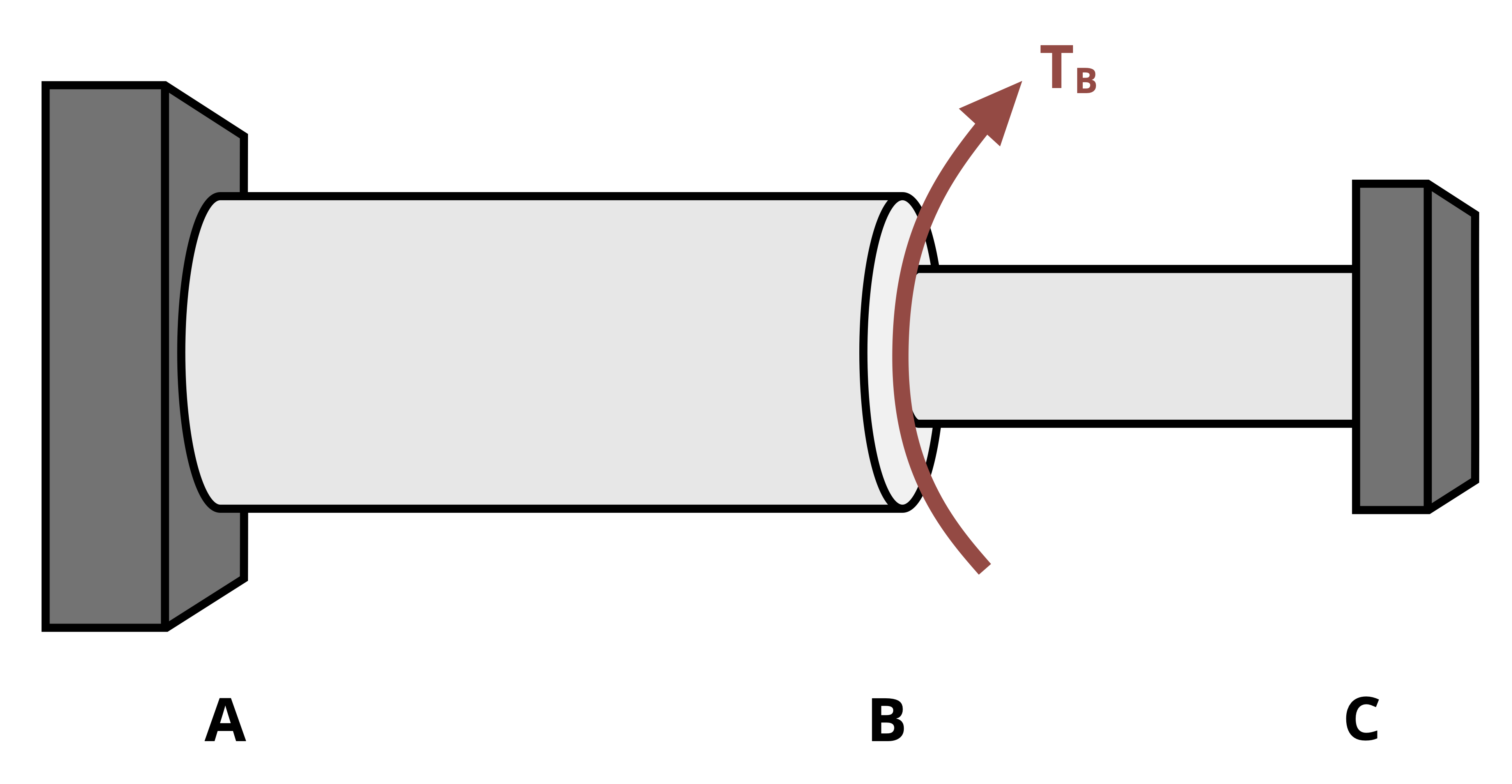
When finding the angle of twist, the angle at any given point along the length of the shaft relative to some reference point. Often the reference point is a fixed point (e.g., at a fixed support), so the relative angle is an absolute angle. In this case, the symbol φ is subscripted with the point along the shaft where the angle was calculated. For example, given the shaft assembly in Figure 6.13, the notation φB denotes the angle of twist at point B relative to the fixed point A.
When finding the relative angle of twist between two nonfixed points on the same shaft section (same T, J, and G), we notate the angle of one point relative to another on the same section by using two subscripts specifying the two points. For example, the angle of twist of D relative to C in Figure 6.13 is notated as φCD. In this case we perform the calculation for the angle of twist at D as if point C is fixed.
\[ \phi_{C D}=\frac{T_{C D} L_{C D}}{J_{C D} G_{C D}} \]
To find the relative angle of twist between two nonfixed points (let’s say B and D in Figure 6.13) that are on different shaft sections (i.e., one or more sections change between them due to changing T, J, or G), sum the angles of twist of each section between them. In this case, the notation would be φD/B, which is the angle of twist of D relative to B. If point C is where the section change occurs, the calculation would be
\[ \phi_{D / B}=\phi_{B C}+\phi_{C D}\text{.} \]
These concepts are illustrated in Example 6.3, which continues with the same bar assembly and loading used in Example 6.1 and Example 6.2.
Example 6.3
The multisection steel bar of Example 6.1 and Example 6.2 is repeated here with the same loading (TB = 70 N·mm and TE= 30 N·mm). The diameters are given as dAC = 50 mm, dCD = 20 mm, and dDE = 35 mm, and section lengths as LAB = 300 mm, LBC = 200 mm, LCD = 400 mm, and LDE = 700 mm. All sections have a shear modulus of G = 40 GPa.
Determine the angle of twist of points C, D, and E, all relative to fixed point A.
A negative result indicates a clockwise twist, and a positive result indicates a counterclockwise twist.
6.5 Statically Indeterminate Torsion
Click to expand
As discussed in Section 5.5 for axial loading, we may sometimes encounter loading and constraint conditions that are statically indeterminate. In these situations, though a structure may be in static equilibrium, equilibrium equations do not provide enough equations to solve for all the unknown reactions. In many cases, the known constraints on deformation can be used to provide the additional necessary equations. Let’s consider the following two types of statically indeterminate problems for torsional loading:
Redundant supports: These are cases where each end has a fixed support. In this configuration, the shaft is constrained on both ends such that the overall angle of twist must be 0 if both ends are truly fixed. As a variation, we could also consider the case where the angle of twist is limited to a specified amount if there is a fixed degree of freedom on one end (for example if one side involves a loose connection).
Example 6.4 demonstrates how to solve a statically indeterminate torsion problem that falls into this category. The example considers both the case where the total angle of twist is 0 and the case where there is a fixed degree of freedom.
Example 6.5 re-examines part (a) of Example 6.4 to demonstrate a different method of solving the problem. This method is known as the method of superposition and is outlined below.
Coaxial or parallel shafts: Multiple shafts are bonded concentrically (one within another) so that they are constrained to twist as a unit by the same amount. In this case, the extra equation needed in addition to equilibrium comes from setting each shaft’s angle of twist equal to the other’s.
Example 6.6 demonstrates how to solve a statically indeterminate torsion problem that falls into this category of loading.
6.5.1 Method of Superposition
For the case of redundant supports, an alternative is to use the method of superposition. The method of superposition is based on the idea that the effects of individual loads on the deformation of a body can be calculated individually and then added together to obtain the total effect. To apply this method do the following:
- Draw the FBD of the whole body and write out the relevant equilibrium equations.
- Choose one of the supports to consider redundant, remove the corresponding reaction torque, and find the total angle of twist from the remaining loads.
- Put the reaction torque from the redundant support back, remove the applied loads, and then find the total angle of twist due to the replaced reaction torque in terms of the corresponding variable.
- Sum the angle of twist from step 2 and step 4 and set the total equal to zero (or a given angle as appropriate).
- Solve the equation resulting from step 4 for the reaction at the redundant support and then use the whole body equilibrium to solve for the reaction at the other support(s).
Example 6.5 demonstrates the use of superposition to solve part (a) of Example 6.4.
Example 6.4
A shaft assembly consists of a 12 in. long steel section AB (d = 10 in., G = 11,600 ksi) bonded rigidly to a 9 in. long solid brass section BC (d = 7 in., G = 5,800 ksi). The assembly is to be bolted to walls A and C.
If a torque TB of magnitude 2,000 kip·in. is applied at B, determine the shear stress in the steel section and the brass section after the ends are bolted for each of the following conditions:
a. Both ends A and C are tightly connected immediately at installation.
b. A slight misalignment exists at end A that necessitates turning that end by 0.5° to lock in.
To calculate stresses, we need to know the internal torque in each section. To find the internal torque, we need to know at least one of the reaction torques exerted by the walls at A and C. The steps below can be used to find the reaction torques.
Step 1: Draw the FBD of the whole body and write the relevant equilibrium equation(s).
In this case the only helpful equilibrium equation is \(\sum M_x=0\).
Note that the assumed directions for TA and TC (the reaction torques exerted by the bolts) would usually be completely assumed, with the signs of the answers indicating if the assumed directions are correct. For case (a), this is still true.
For case (b) we must be more careful. The direction of the 0.5° turn is not specified, but it must be in the direction of TB, since that is the only applied load. The direction of TA, which is the reaction torque exerted by the bolt at A, should be in the direction opposite to the way the shaft turns since the bolt is there to fix the assembly in place.
The assumed direction of TC can be in either direction for both case (a) and case (b).
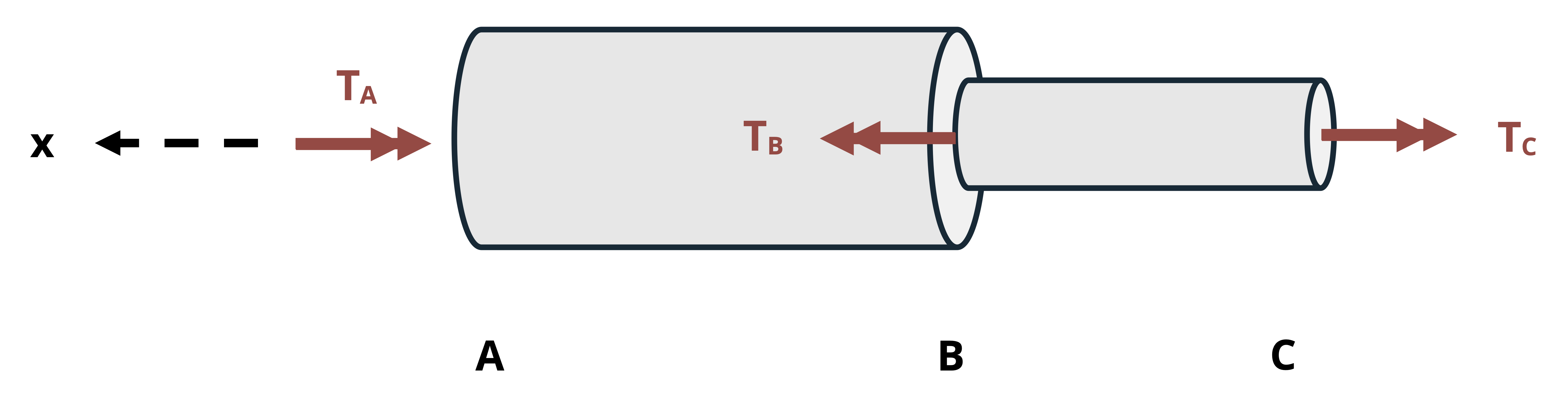
The positive x-axis goes from right to left in the whole body FBD. As long as the choice of signs applied to torques for any whole body equation is based on the same assumption, it does not matter which direction is chosen to be the positive x direction. In this case, the signs on the torques will be based on the way the torques are perceived when looking in the direction from A towards C.
Since the direction of TB is counterclockwise from that perspective, it is drawn in the positive x direction. TA is drawn in the negative x direction. TC is arbitrarily assumed to be the same direction as TA. Write the moment equilibrium equation.
\[ \begin{gathered} \sum M_x=-T_A+T_B-T_C=0 \\ T_C+T_A=T_B \end{gathered} \]
Because there are two unknowns (TA and TC) but only one equilibrium equation, the problem is statistically indeterminate.
Step 2: Apply kinematic constraint.
Applying the kinematic constraint will provide the second equation needed to solve for TA and TC. For case (a), both ends are fixed at the time of installation so the total angle of twist should be zero. Thus
\[ \phi=\sum \frac{T L}{J G}=\phi_{A B}+\phi_{B C}=0\text{.} \]
For case (b), the misalignment means end A must be turned by 0.5° before it gets locked in, so the magnitude of the total angle of twist is also 0.5°. In step 1, it was discussed that the twist will be in the same direction as TB, which is counterclockwise looking from A toward C.
So for case (b), the kinematic equation is
\[ \phi=\sum \frac{TL}{JG}=\phi_{A B}+\phi_{BC}=+0.5^{\circ} * \frac{\pi}{180^{\circ}}\text{.} \]
Step 3: Write the compatibility equation.
Write the compatibility equation by substituting the appropriate torque-twist equations (Equation 6.2) for the angles of twist in the kinematic constraint equation.
To implement this step, establish the internal torque (and sign) for each section by cutting sections and applying equilibrium.
The FBD for a section made by cutting through section AB is as shown.
The equilibrium equation for this section is
\[ \sum M_x=T_A+T_{A B}=0\\ T_{AB}=-T_A\text{.} \]
Thus, the angle of twist in section AB is
\[ \phi_{AB}=\frac{T_{AB}L_{AB}}{J_{AB}G_{AB}}=\frac{-T_A*(12{~in.})}{\frac{\pi}{32}(10{~in.})^4*(11,600{~ksi})}\text{.} \]
The FBD for a section made by cutting through section BC is as shown.
The equilibrium equation for this section is
\[ \sum M_x=-T_{B C}+T_C=0\\ T_{BC}=T_C\text{.} \]
The angle of twist in section BC is
\[ \phi_{B C}=\frac{T_{BC}L_{BC}}{J_{BC}G_{BC}}=\frac{T_C*(9{~in.})}{\frac{\pi}{32}(7{~in.})^4*(5,800{~ksi})}\text{.} \]
Substituting the expressions for φAB and φBC into the kinematic constraint equation for case (a) gives the compatibility equation
\[ \frac{-T_A*(12{~in.})}{\frac{\pi}{32}(10{~in.})^4*(11,600{~ksi})}+\frac{T_C*(9 {~in.})}{\frac{\pi}{32}(7{~in.})^4*(5,800{~ksi})}=0\text{.} \]
Case (b) gives the compatibility equation
\[ \frac{-T_A*(12{~in.})}{\frac{\pi}{32}(10{~in.})^4*(11,600{~ksi})}+\frac{T_C*(9 {~in.})}{\frac{\pi}{32}(7{~in.})^4*(5,800{~ksi})}=0.5^{\circ}*\frac{\pi}{180^{\circ}}\text{.} \]
Step 4: Solve the equilibrium and compatibility equations simultaneously for TA and TC.
Case (a):
\[ \begin{aligned} &T_A=T_C\left[\frac{9{~in.}*\frac{\pi}{32}(10{~in.})^4*(11,600{~ksi})}{12{~in.}*\frac{\pi}{32}(7{~in.})^4*(5,800{~ksi})}\right] \\ \\ &T_A=T_C[6.247] \\ \\ &\text{Substitute into}~T_A+T_C=2,000{~kip}\cdot{in.} \\ \\ &6.247T_C+T_C=2,000{~kip}\cdot{in.} \\ \\ &T_C=276{~kip}\cdot{in.} \\ &T_A=1,724{~kip}\cdot{in.} \end{aligned} \]
Case (b):
\[ \begin{aligned} &T_A=\left(\frac{T_C*(9{~in.})}{\frac{\pi}{32}(7{~in.})^4*(5,800{~ksi})}-0.5^\circ*\frac{\pi}{180^\circ}\right)*\left(\frac{\frac{\pi}{32}(10{~in.})^4*11,600{~ksi}}{12~in.}\right) \\ \\ &T_A=T_C[6.247]-8,282{~kip}\cdot{in.} \\ \\ &\text{Substitute into}~T_A+T_C=2,000{~kip}\cdot{in.} \\ \\ &6.247T_C+T_C-8,282{~kip}\cdot{in.}=2,000{~kip}\cdot{in.} \\ \\ &T_C=1,419{~kip}\cdot{in.} \\ &T_A=581{~kip}\cdot{in.} \end{aligned} \]
The results are positive for both cases, so the assumed directions are the actual directions.
Step 5: Calculate stresses.
Now that the reaction torques are known and it was established in step 3 that TAB = TA and TBC = TC in magnitude, the shear stresses in the two sections can be calculated using Equation 6.1.
Case (a):
\[ \begin{aligned} & \tau_{AB}=\frac{T_{AB}*c_{AB}}{J_{AB}}=\frac{1,724{~kip}\cdot{in.}(5{~in.})}{\frac{\pi}{32}(10{~in.})^4}=8.78{~ksi} \\ & \tau_{BC}=\frac{T_{BC}*c_{BC}}{J_{BC}}=\frac{276{~kip}\cdot{in.}(3.5{~in.})}{\frac{\pi}{32}(7{~in.})^4}=4.10{~ksi} \end{aligned} \]
Case (b):
\[ \begin{aligned} & \tau_{AB}=\frac{T_{AB}*c_{AB}}{J_{AB}}=\frac{581{~kip}\cdot{in.}*5{in.}}{\frac{\pi}{32}(10{~in.})^4}=2.96{~ksi} \\ & \tau_{BC}=\frac{T_{BC}*c_{BC}}{J_{BC}}=\frac{1,419{~kip}\cdot{in.}*3.5{~in}}{\frac{\pi}{32}(7{in.})^4}=21.1{~ksi} \end{aligned} \]
Answer:
Case (a): τAB = 8.78 ksi, τBC = 4.10 ksi
Case (b): τAB = 2.96 ksi, τBC = 21.1 ksi
Example 6.5
Solve part (a) of Example 6.4 using the method of superposition. The problem statement is repeated here for convenience.
A shaft assembly consisting of a 12 in. long steel section AB (d = 10 in., G = 11,600 ksi) is bonded rigidly to a 9 in. long solid brass section BC (d = 7 in., G = 5,800 ksi). The assembly is bolted to walls A and C.
If both ends A and C are tightly connected to the walls and a torque TB of magnitude 2,000 kip·in. is applied at B, determine the shear stress in the steel section and the brass section.
The first step to solving (global equilibrium) remains the same. The method of superposition is applied in step 2 and step 3.
Step 1: Draw the FBD of the whole body and write out the relevant equilibrium equations.
Draw the whole body FBD and write out the relevant equilibrium equations. Shown on the FBD are the assumed directions for TA and TC as well as the direction used for the positive x direction. Recall that the direction of the torque should be determined by looking from the positive x-axis toward the negative (A to C).
Applying equilibrium in this case reduces to the sum of the moments about the x-axis as the only nontrivial equation.
\[ \begin{gathered} \sum M_x=-T_A+T_B-T_C=0 \\ T_C+T_A=T_B \end{gathered} \]
Because there are two unknowns (TA and TC) but only one equilibrium equation, the problem is statically indeterminate.
Step 2: Choose one of the supports to consider redundant, remove the corresponding reaction torque, and then find the total angle of twist from the remaining loads.
Let’s consider the support at C to be redundant. Note that the support at A could alternatively be considered redundant with the same results.
With no support at C, a section cut within BC shows that the internal torque TBC must be 0 for equilibrium.
A section cut through AB shows that the internal torque TAB = TB with the direction of TAB opposite of TB. Viewed from the cut towards C, TB is counterclockwise, so TAB is clockwise. Therefore, the angle of twist is negative and equal to
\[
\phi_{C/A}=\sum \frac{TL}{JG}=-\frac{T_{AB}L_{AB}}{J_{AB} {G}_{AB}}=-\frac{(2,000{~kip}\cdot{in.})*(12{~in.})}{\frac{\pi}{32}(10{in.})^4*(11,600{~ksi})}=-2.107 \times 10^{-3}{~rad}
\]
Step 3: Put the reaction torque from the redundant support back, remove the applied loads, and then find the total angle of twist due to the replaced support torque in terms of the corresponding variable.
The section FBDs in this case reveal that both TAB and TBC are equal in magnitude and opposite in direction from TC. Since both are pointed away from the cut, the direction is taken to be counterclockwise, or positive. So the angle of twist with this loading is
\[
\begin{aligned}
\phi_{C/A}&=\sum\frac{TL}{JG}=\frac{T_{AB}L_{AB}}{J_{AB}{G}_{AB}}+\frac{T_{BC}L_{BC}}{J_{BC}G_{BC}} \\
\\
&=\frac{T_C*(12{~in.})}{\frac{\pi}{32}(10{~in.})^4*(11,600{~ksi})}+\frac{T_C*(9{~in.})}{\frac{\pi}{32}(7{~in.})^4*(5,800{~ksi})} \\
\\
&=7.637\times 10^{-6}~T_{C}
\end{aligned}
\]
Step 4: Set the sum of the angles of twist equal to 0 (or other fixed angle when applicable) and solve for the unknown reaction torque.
The total angle of twist should be equal to zero when the ends are tightly bolted to the walls without extra twisting.
\[ 2.107 \times 10^{-3}{~rad}+7.637 \times 10^{-6}~T{c}=0 \]
Solving for TC gives TC = 276 kip·in which is the same result found in Example 6.4.
Step 5: Use the whole body equilibrium equation from step 1 to solve for the other reaction torque.
Substituting the above result for TC into the whole body equilibrium equation from step 1 gives TA = 1,724 kip in as was found in Example 6.4. Once again the corresponding shear stresses are
\[ \begin{aligned} & \tau_{AB}=\frac{T_{AB}*c_{AB}}{J_{AB}}=\frac{1,724{~kip}\cdot{in.}*5{~in.}}{\frac{\pi}{32}(10{~in.})^4}=8.78{~ksi} \\ & \tau_{BC}=\frac{T_{BC}*c_{BC}}{J_{BC}}=\frac{276{~kip}\cdot{in.}*3.5{~in.}}{\frac{\pi}{32}(7{~in.})^4}=4.10{~ksi} \end{aligned} \]
Answer:
τAB = 8.78 ksi
τBC = 4.10 ksi
Example 6.6
The vertical shaft assembly is fixed to the bottom surface and consists of a solid brass (G = 40 GPa) circular shaft completely bonded in section BC to a steel (G = 80 GPa) reinforcing tube. The diameter of the brass is 25 mm along the whole length, and the outer diameter of the steel is 50 mm. The assembly is subjected to torques TB = 800 N·m and TA = 300 N·m in the directions shown.
Determine the magnitude of the shear stress in the brass in sections AB and BC.
First we’ll find the shear stress in the brass in section BC. To begin, we determine how much of the internal torque within that section is supported by the brass versus how much is supported by the steel.
Step 1: Draw the FBD of a section cut through BC to examine the internal torque in BC.
Since the reaction at C is not strictly necessary to solve this problem, the whole body FBD is not needed here. Start by cutting a section through BC and drawing the FBD. Note that instead of representing the internal reaction at the cut as TBC, it is split into the components that make up TBC: TBr and TSt.
With only one nontrivial equilibrium equation (\(\sum M_x=0\)) and two unknowns, the problem is statically indeterminate.
\[ \sum M_x=T_A-T_B-T_{Br}-T_{St}=0 \]
Step 2: Apply the kinematic constraint to obtain a second equation.
In this case, the materials are fully bonded in section BC, so the materials are constrained to twist as a unit in that section. In section BC, the kinematic equation is
\[ \phi_{B r}=\phi_{s t}\text{.} \]
Step 3: Substitute the torque-twist equation into the kinematic equation to get the compatibility equation.
Substituting Equation 6.2 into the kinematic constraint equation gives us a second equation that relates TBr and TSt.
\[ \frac{T_{Br}L_{Br}}{J_{Br}G_{Br}}=\frac{T_{St}L_{St}}{J_{St}G_{St}} \]
The lengths are equal and therefore cancel each other. Rearrange this equation to get an expression for TSt in terms of TBr.
\[ \begin{aligned} T_{St}&=\frac{T_{Br}J_{St}G_{St}}{J_{Br}G_{Br}} \\ \\ &=T_{Br}\left[\frac{\frac{\pi}{32}\left((0.05{~m})^4-(0.025{~m})^4\right)\left(80 \times 10^9~\frac{{N}}{{m}^2}\right)}{\frac{\pi}{32}(0.025{~m})^4\left(40 \times 10^9 \frac{{N}}{{m}^2}\right)}\right] \\ \\ &=30.0~T_{Br} \end{aligned} \]
Step 4: Use the equilibrium equation and the simplified compatibility relationship to solve for TBr.
Substite Tst = 30 TBr into the equilibrium equation.
\[ \begin{aligned} & 300{~N}\cdot{m}-800{~N}\cdot{m}-T_{Br}-30~T_{Br}=0\\[10pt] & T_{Br}=-16.1 {~N}\cdot{m} \end{aligned} \]
Step 5: Apply the torque-shear stress equation to find the shear stress in the brass for sections AB and BC.
Note that because only the magnitude of the stress is requested, we substitute torque values in as positive values.
Applying Equation 6.1 in section BC yields
\[ \tau_{Br(B C)}=\frac{(T_{Br})(c_{Br})}{J_{Br}}=\frac{(16.1{~N}\cdot{m})(0.0125{~m})}{\frac{\pi}{32}(0.025{~m})^4}=5.26{~MPa}\text{.} \]
In section AB, which consists only of brass, all the internal torque is carried by the brass. Making a cut within that section and applying equilibrium shows that the magnitude of the internal torque TAB = TA = 300 N·m.
Applying the shear stress equation yields
\[ \tau_{Br(AB)}=\frac{(T_{Br})(c_{Br})}{J_{Br}}=\frac{(300{~N}\cdot{m})(0.0125{~m})}{\frac{\pi}{32}(0.025{~m})^4}=97.8{~MPa}\text{.} \]
Answer:
τBr in section BC is 5.26 MPa
τBr in section AB is 97.8 MPa
6.6 Power Transmission
Click to expand
As mentioned in the introduction to torsion, one common application where we encounter circular shafts subjected to torsion is in power transmission shafts. In these types of assemblies, shafts are connected and apply torque to one another through gears and belts. If a shaft somewhere in the assembly is connected to a motor that causes it to rotate, that rotation is then transmitted to other connected shafts, which can in turn transmit rotation to even more shafts. Note that such systems are considered to be in equilibrium even with the rotation as long as the angular velocity remains constant.
Below is a brief derivation of the equation that relates torque to power, followed by a discussion of how torque and angle of twist are affected by the gear or belt connections between shafts.
6.6.1 Derivation of Power-Torque Relationship
Recall from other subjects of study that power is defined to be the time rate of change of work. The definition of work is force times distance. So power can be calculated as
\[ P=\frac{W}{t}=\frac{F \times d}{t}\text{.} \]
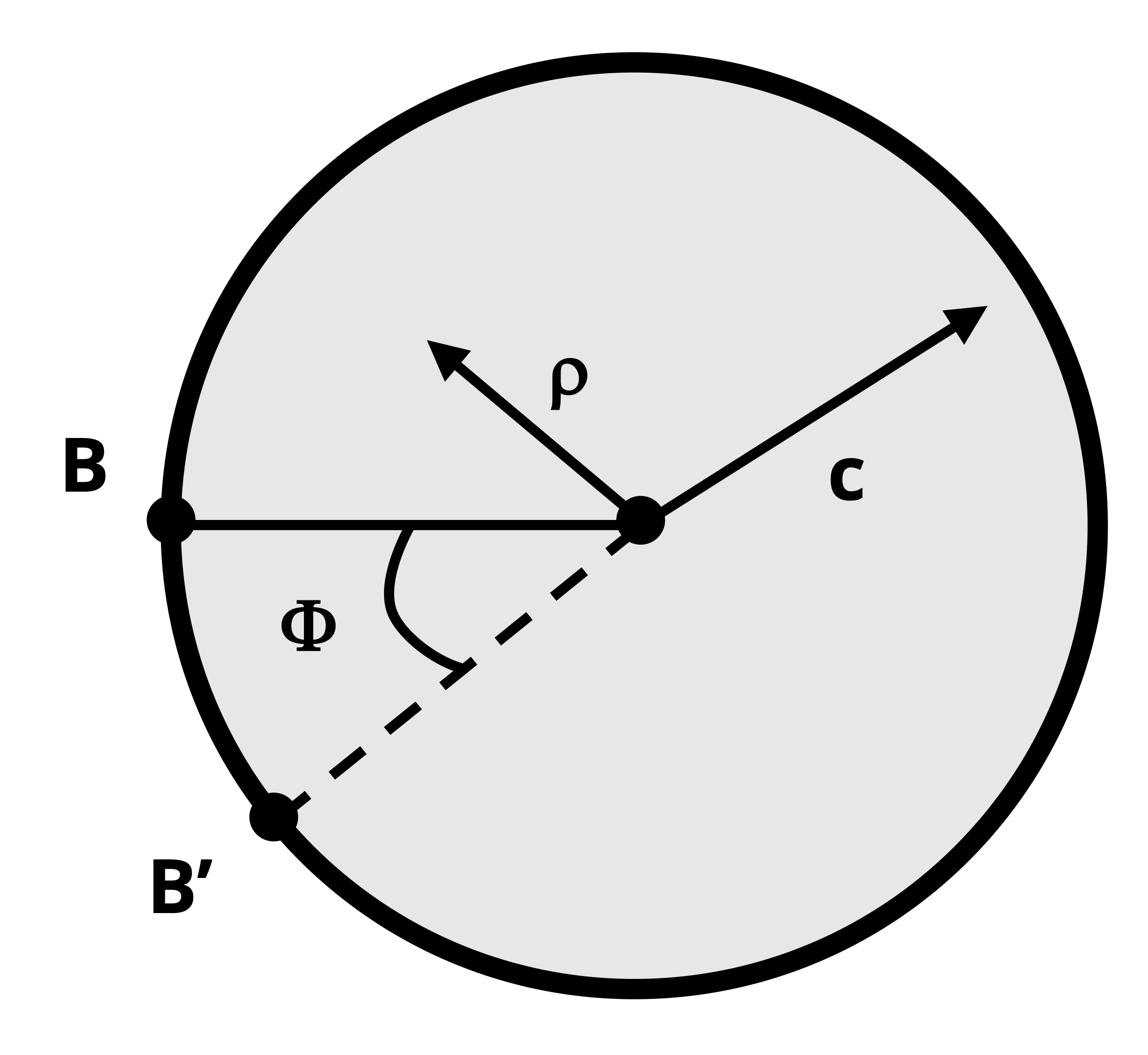
Within the context of rotating shafts, the force is applied to the shaft’s outer edge resulting in torque, and the distance is the arc length of a point on the shaft’s edge that travels around the circumference in a given amount of time, t. Figure 6.14 illustrates this point.
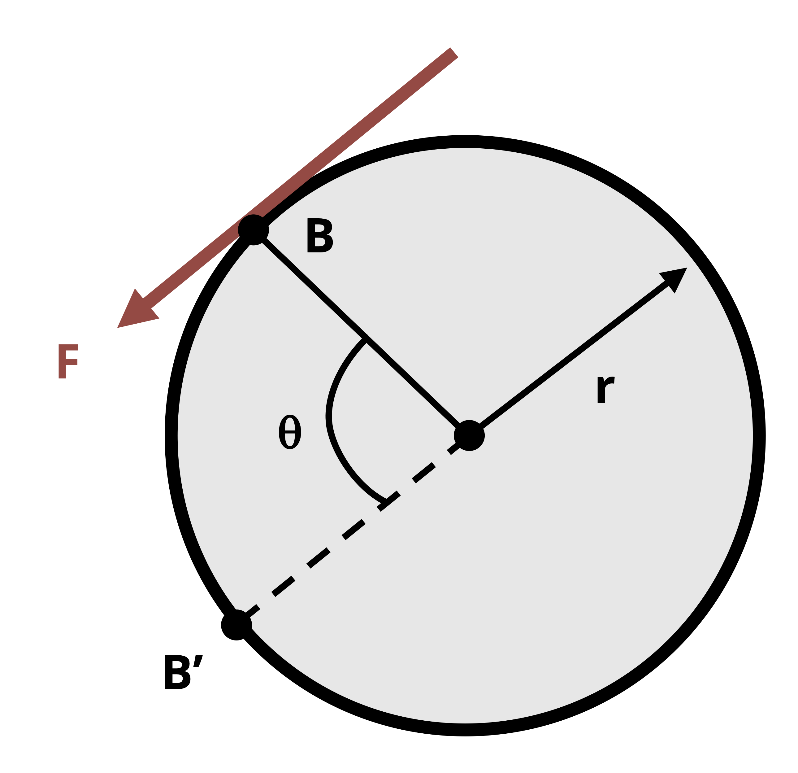
If the arc length over which point B travels is BB’ = rθ, then W = F(rθ). Since torque is equal to (F)(r), we can see that W = Tθ. Substituting this expression for work into the power equation above, we then have \(P=\frac{T \theta}{t}\). The \(\frac{\theta}{t}\) term is angular velocity, which is denoted here with the Greek letter ω. So the power equation can finally be expressed as
\[ \boxed{{P = T\omega}}\text{ ,} \tag{6.3}\]
P = Power [Watts, in.-lb/sec, horsepower]
T = Torque [N·m, lb·in.]
𝜔 = Angular velocity [rad/s, rad/sec]
6.6.2 Units
In SI the standard unit for power is the Watt (W), which is (N·m)/s. The N·m unit is also referred to as a Joule, so a Watt is a Joule/s.
In US customary units, power is commonly expressed as ft·lb/s or in.·lb/s. However, it is also common to express power in terms of horsepower, where 1 hp = 550 ft·lb/s. Note that there is a conversion difference between US horsepower and British horsepower. In this text, horsepower refers to the US version.
In applying Equation 6.3, the angular velocity ω must be expressed in radians per second. Sometimes angular velocity is given in Hz, where 1 Hz = 1 revolution/s. In this case, one must use the fact that 1 revolution = 2π radians to convert from Hz to rad/s. If angular velocity is given in revolutions per minute (rpm), then we must multiply by 2π radians and also divide by 60 to convert 1/min to 1/s. This reduces to an overall multiplication factor of π/30 to convert from rpm to rad/s.
A summary of the power related units and conversions is provided in Table 6.1 and Table 6.2.
Table 6.1: Power units
| SI (watt) | \[ W=\frac{N m}{s}=\frac{J}{s} \] |
| US | \[ \left(\frac{f t\ l b}{s}\right) \operatorname{or}\left(\frac{in.\ l b}{s}\right) \] |
| US (horsepower, hp) | \[ 1\ h p=\frac{550 f t\ l b}{s} \] |
| Hertz (Hz) | \[ 1\ H z=1 \frac{r e v}{s} \] |
| Angular velocity given Hz (rad/s) | \[ 1 \frac{rev}{sec}\ (2\pi \frac {rad}{rev})=\frac {2\pi \frac{rad}{s}}{Hz} \] |
| Angular velocity given rpm (rad/s) | \[ 1\frac{r e v}{\min }\left(\frac{2 \pi\ \mathrm{rad}}{1\ \mathrm{rev}}\right)\left(\frac{1 \mathrm{~min}}{60 \mathrm{~s}}\right)=\frac {\frac {\pi}{30}\frac {rad}{s}}{rpm} \] |
6.6.3 Torque Transfer Between Connected Gears (Gear Ratio)
Consider two connected gears such as shown in Figure 6.15. The interaction of the teeth results in a force applied to each gear from one gear to the other. For equilibrium, this force must be equal in magnitude but opposite in direction. The force results in a torque that can be expressed as T = Fr.
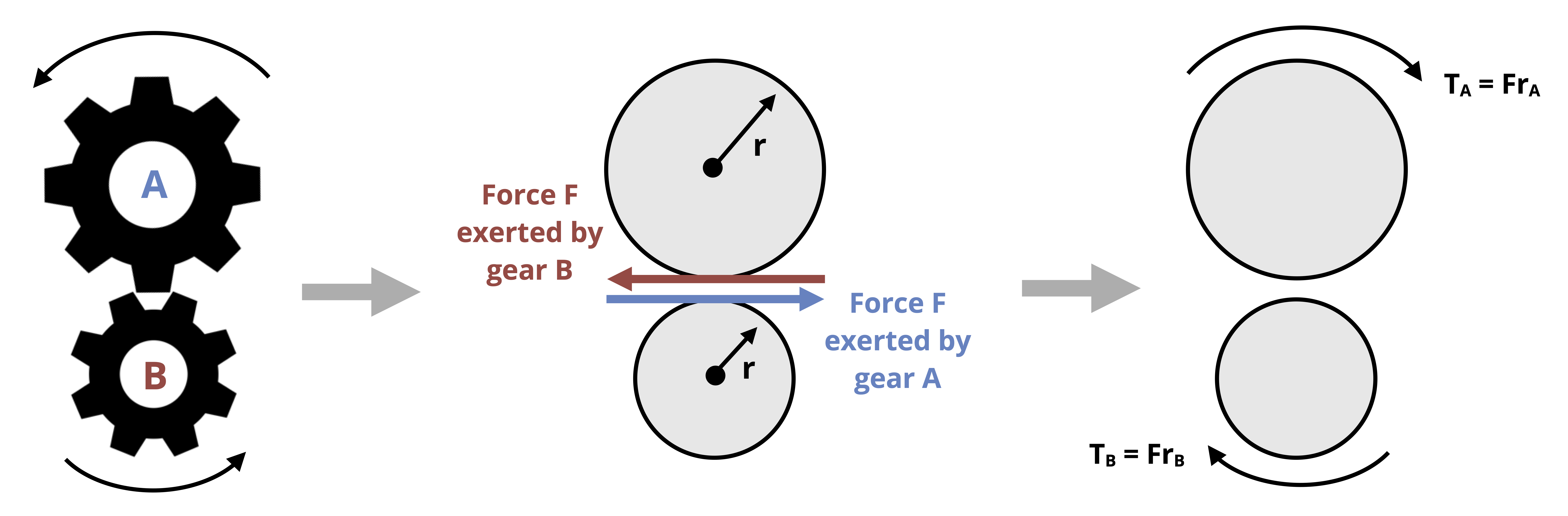
Given that the force on each gear is equal in magnitude to the force on the other in equilibrium, we can write
\[ F=\frac{T_A}{r_A}=\frac{T_B}{r_B}\text{,} \]
which then allows us to express the torque exerted by one gear in terms of the torque exerted by the other as well as the ratio of radii.
\[ \boxed{{T_A=\frac{r_A}{r_B} T_B}} \tag{6.4}\]
The ratio of radii is known as the gear ratio. It can also be expressed as the ratio of gear diameters (\(\frac{d_A}{d_B})\) or the number of teeth on each gear (\(\frac{N_A}{N_B})\).
While the forces that result in torque are opposite in direction for each gear of the connected pair, the torques themselves are in the same direction. In Figure 6.15, the rightwards force gear A exerts on gear B results in a clockwise torque on gear B. Likewise, the leftward force gear B exerts on gear A results in a clockwise torque on gear A.
6.6.4 Angular Velocity Ratio of Connected Shafts
When two shafts are connected by a pair of gears, conservation of energy dictates that the power transferred into one shaft equals the power transferring out of the other (power in = power out, assuming losses are negligible).
For two connected gears A and B, if PA = TAωA and PB = TBωB and PA = PB, then \(\omega_A=\frac{T_B}{T_A} \omega_B\).
Substituting in Equation 6.4 gives us
\[ \boxed{{\omega_A=\frac{r_B}{r_A} \omega_B}}\text{ .} \tag{6.5}\]
Note that the gear ratio in this case is inverse of the one used to relate torques.
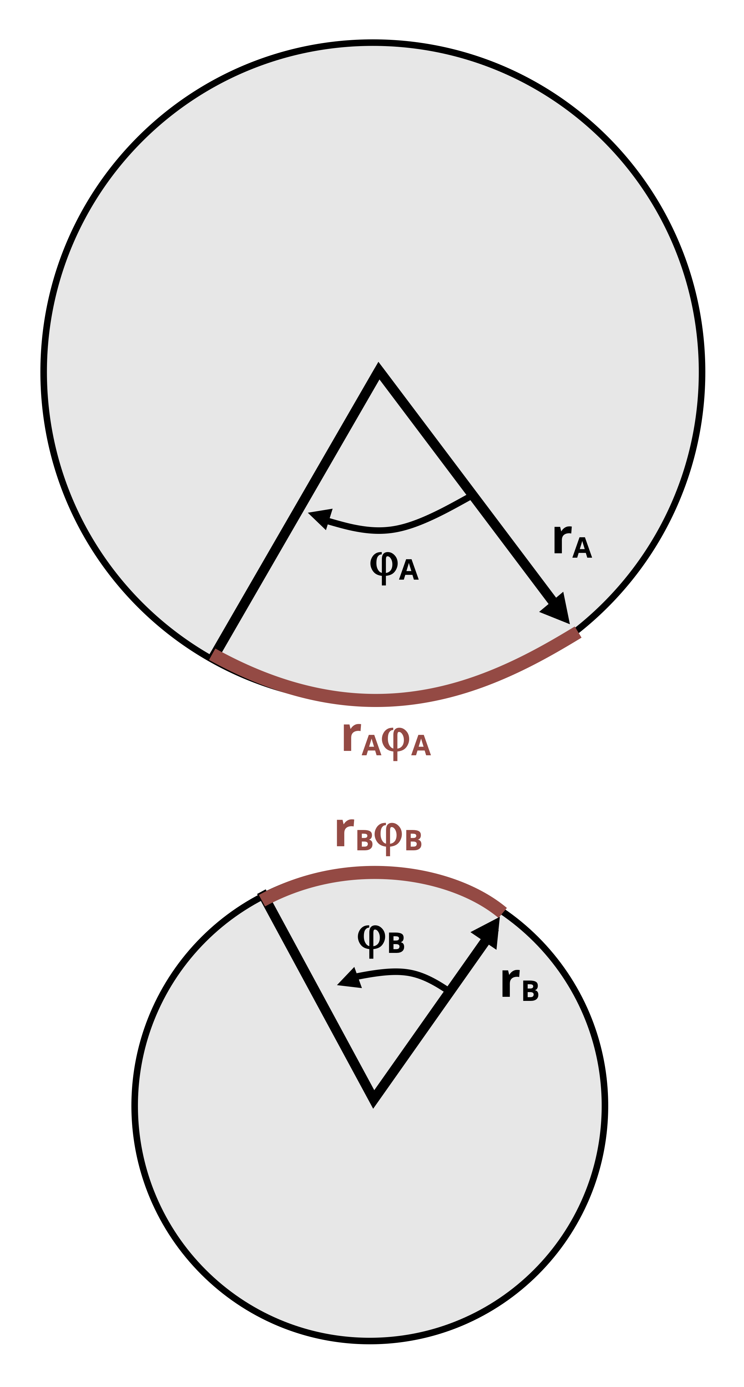
6.6.5 Angle of Twist
When two connected gears, each attached to a separate shaft, rotate they travel the same distance for a given amount of shaft rotation, or angle of twist. The distance of travel is equal to the arc length r·φ. Given that the gears exert forces in opposite directions (as illustrated in Figure 6.15), the direction of travel of each gear will also be opposite of the other, as depicted in Figure 6.16. For connected gears A and B, attached to shafts A and B respectively this can be expressed as
\[ {r_A\phi_A = -r_B\phi_B} \]
where φA is the angle of twist of shaft A and φB is the angle of twist of shaft B. Rearranging this relationship gives
\[ \boxed {\phi_A=-\frac{r_B}{r_A} \phi_B} \tag{6.6}\]
As with the angular velocities, the gear ratio is the inverse of that used to relate torques.
Example 6.7 presents a problem of power transmission with connected gears that utilizes the above concepts.
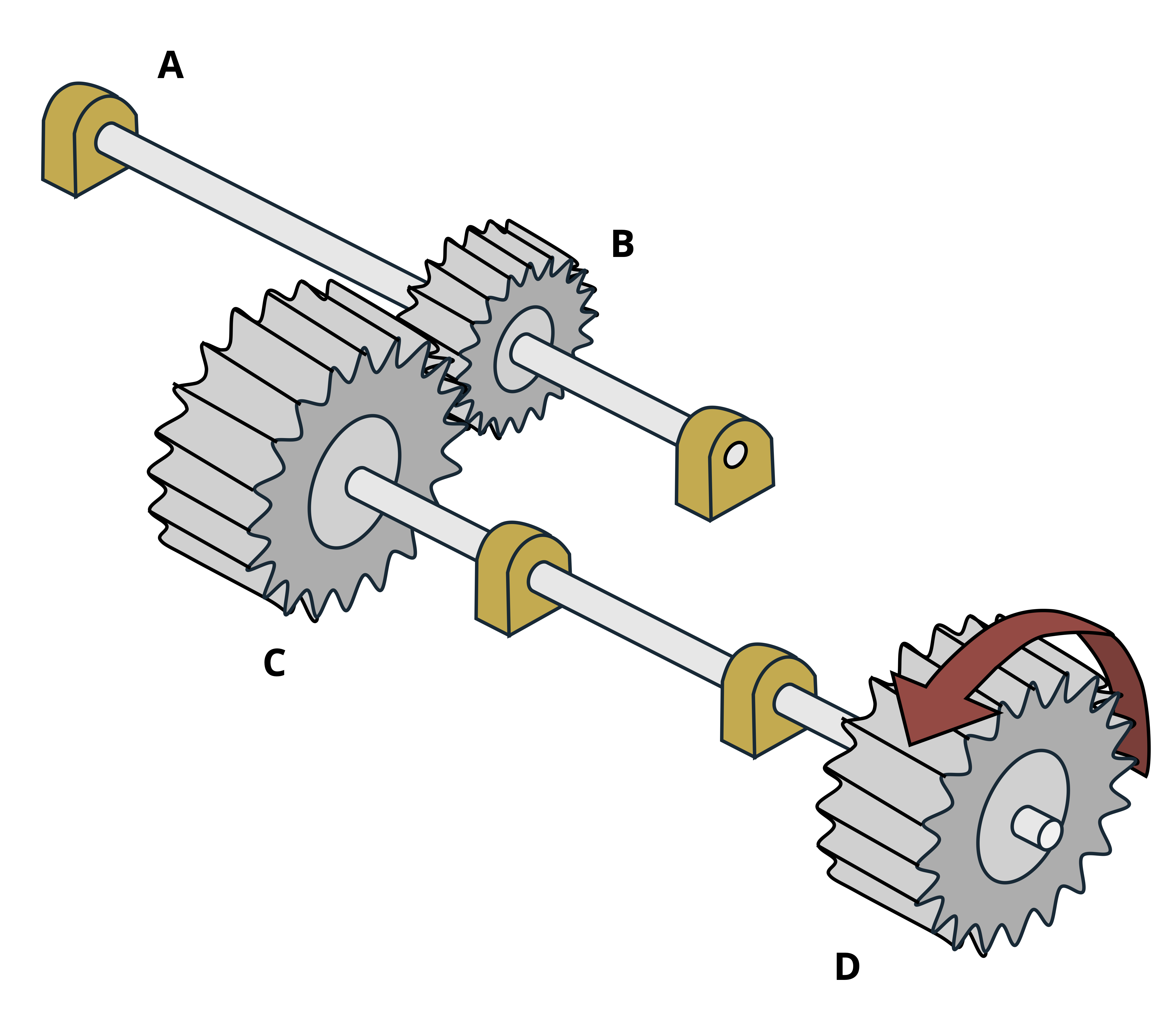
Example 6.7
Power of 60 kW is transmitted at 33 Hz to gear D of the assembly. Shaft CD is allowed to turn freely within its bearings in the direction shown at D. End A of shaft AB is attached rigidly to the wall.
Determine the angle of twist of point D relative to A.
Assume gear C has 35 teeth (NC = 25) around its circumference and gear B has 50 teeth (NB= 50). In addition, shaft AB (d = 40 mm) is 450 mm long and shaft CD (d = 30 mm) is 700 mm long. Both shafts are made of steel (G = 80 GPa).
In general, think of the angle of twist at D as equal to whatever the angle of twist of point C is plus the angle of twist of shaft CD.
\[ \phi_{D / A}=\phi_C+\phi_{C D} \]
With the connection of gear C to gear B, we have
\[ \phi_C=-\frac{r_B}{r_A}\phi_B = -\frac{N_B}{N_A}\phi_B\text{,} \]
so
\[\phi_{D / A}=-\frac{N_B}{N_A}\phi_B+\phi_{C D}\text{.} \]
With NB and NA given, we need to find φB and φCD.
Step 1. Given the power information, calculate the torque applied at D. When considering units, recall that a Watt is an N m/s and a Hz is a revolution per second.
\[
T_D=\frac{P_D}{\omega}=\frac{60,000{~W}}{33{~Hz}\left(\frac{2\pi{~rad}}{{Hz}}\right)}=289.4{~N}\cdot{m}
\]
Step 2. Given the torque at D, calculate the torque at C by applying equilibrium to shaft CD.
\[\sum M_x=T_D-T_C=0 \\ T_C=T_D \]
Looking from D toward C, note that the given direction of TD is counterclockwise, so TC = 289.4 N·m (clockwise).
Step 3. Use the gear ratio to relate the torque exerted on gear C to the torque exerted on gear B. Recall from the discussion in Section 6.6.3 that TB will be the same direction as TC.
\[
T_B=\frac{N_B}{N_C} T_c=\frac{50}{35}(289.4{~N}\cdot{m})=413.4{~N}\cdot{m}\ (clockwise)
\]
Step 4. Calculate φB = φAB (since point A is fixed).
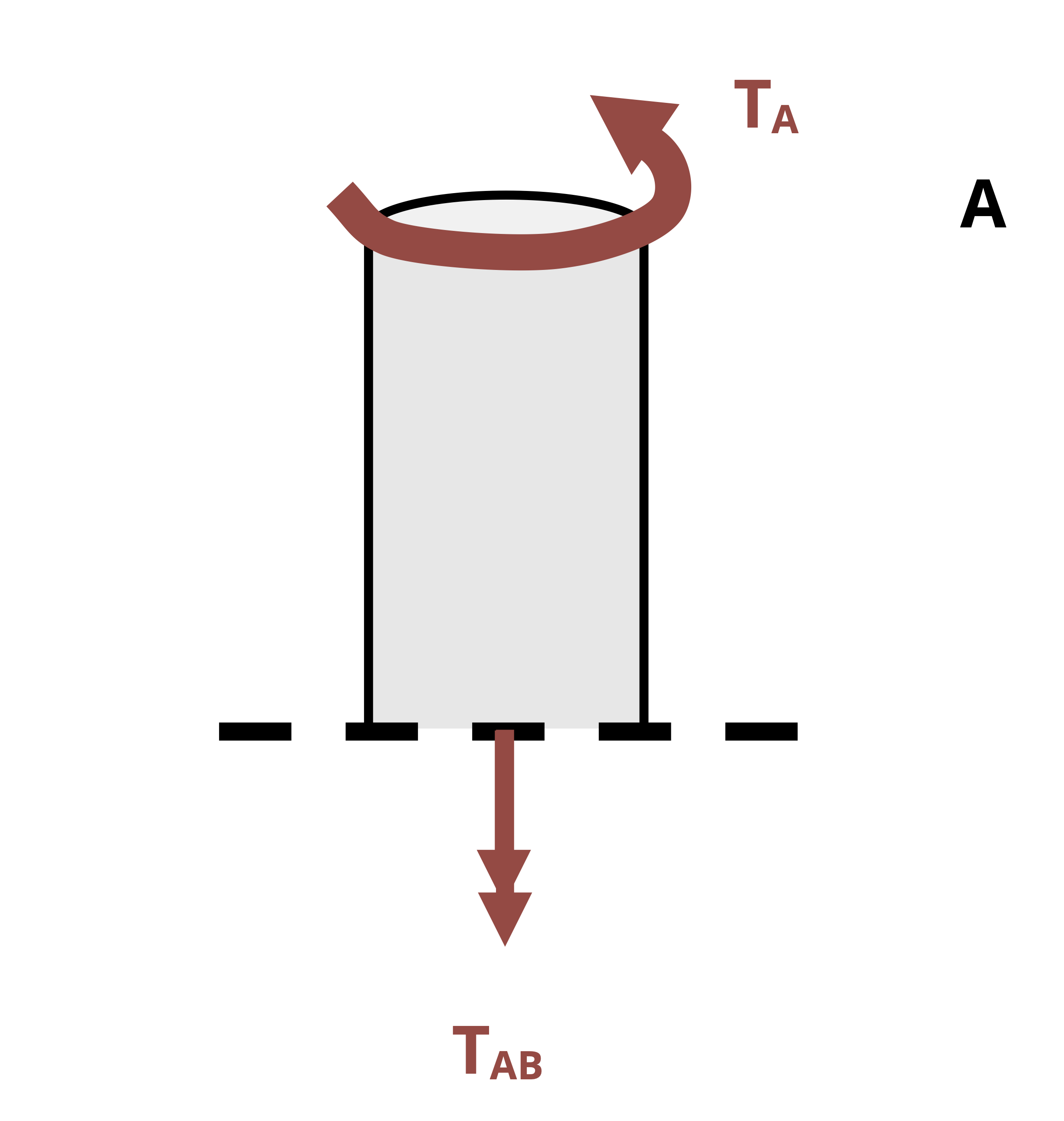
We can see from applying equilibrium to the FBD of a section cut through shaft AB that the internal torque TAB = TB (clockwise). This means that TAB results in a clockwise (negative) angle of twist φAB.
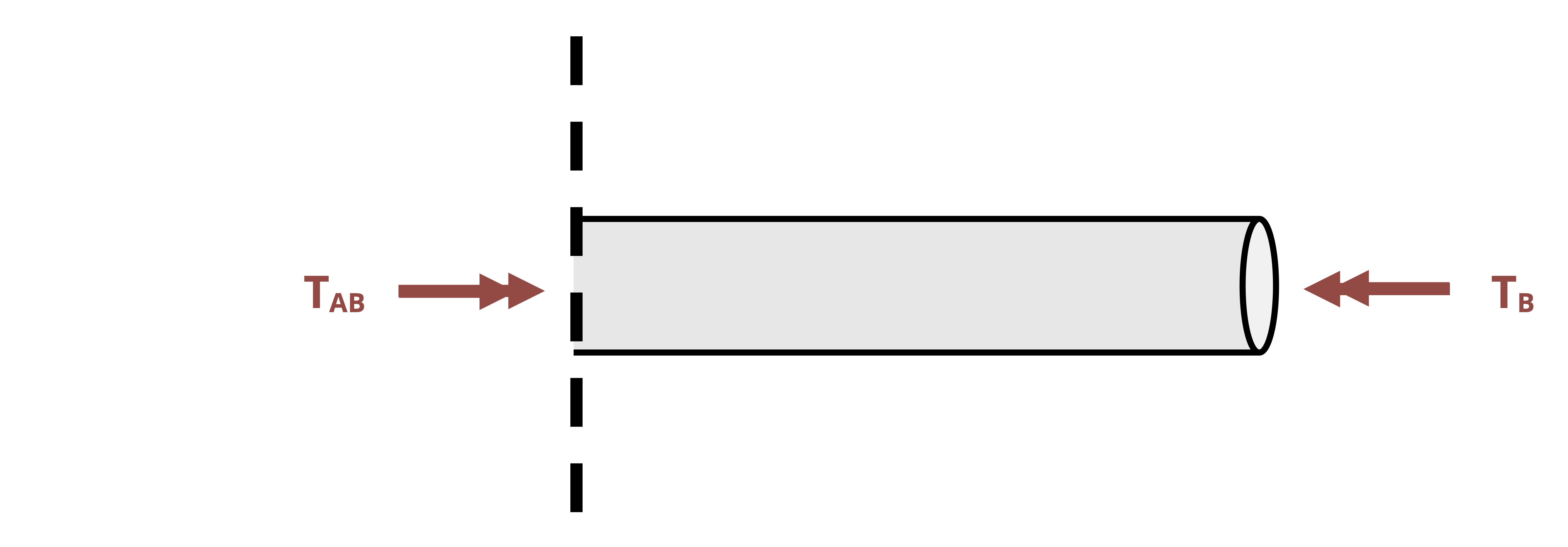
\[
\phi_B=\frac{T_{AB}L_{AB}}{J_{AB}G_{AB}}=-\frac{413.4{~N}\cdot{m}*(0.450{~m})}{\frac{\pi}{32}(0.04{~m})^4\left(80 \times 10^9~\frac{{N}}{{m}^2}\right)}=-0.009252{~rad}
\]
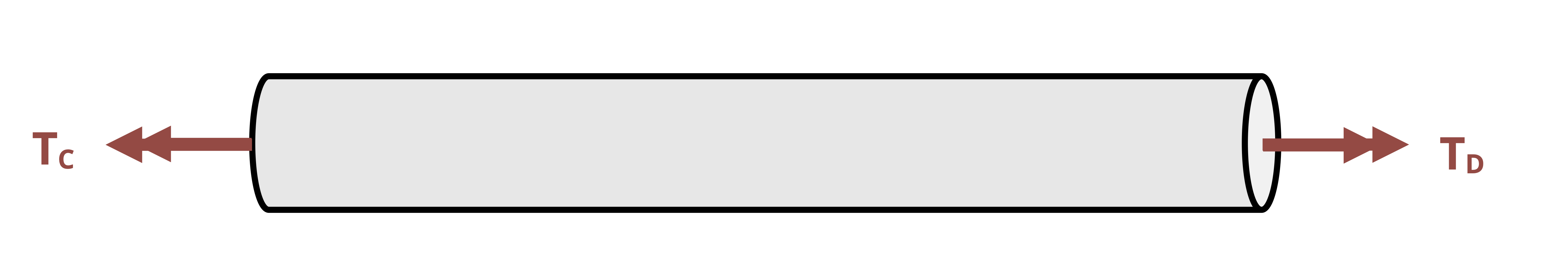
Step 5. Determine and use the internal torque TCD to determine φCD.
Cutting a section through shaft CD and drawing the FBD shows that TCD = TD (counterclockwise), so
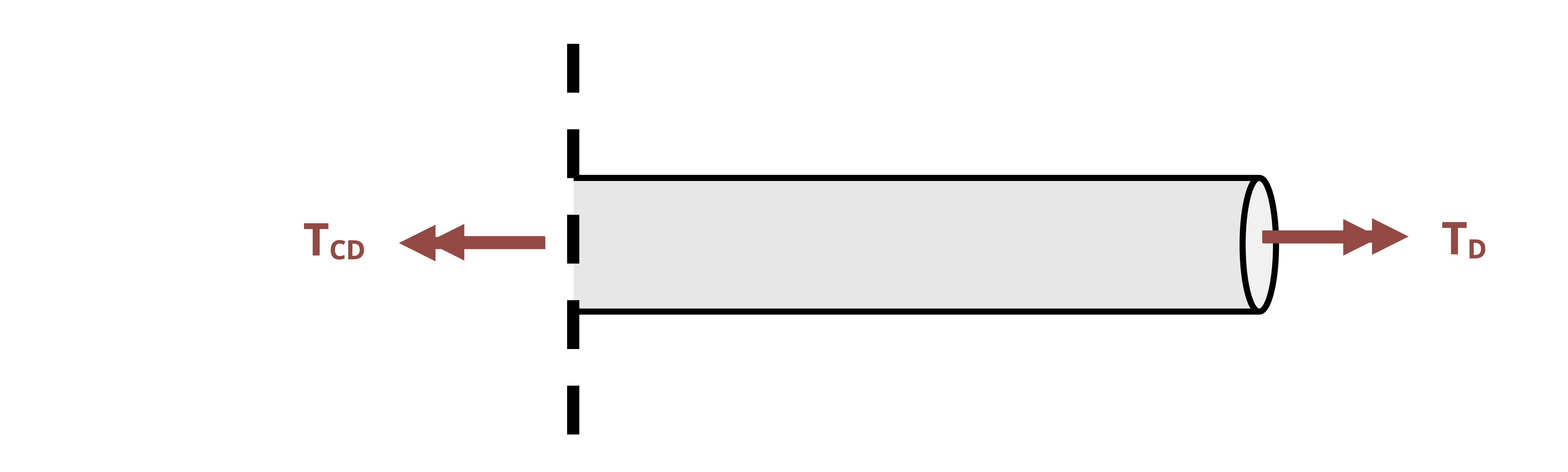
\[
\phi_{C D}=\frac{T_{CD}L_{CD}}{J_{CD}G_{CD}}=\frac{289.4{~N}\cdot{m}*(0.700 {~m})}{\frac{\pi}{32}(0.03{~m})^4\left(80 \times 10^9~\frac{{N}}{{m}^2}\right)}=0.03184{~rad}
\]
Step 6. Calculate \(\phi_{D / A}= -\frac{N_B}{N_A}\phi_B+\phi_{C D}\).
\[
\phi_{D/A}=-\frac{50}{35}(-.009252{~rad})+0.03184{~rad}=0.04506{~rad}
\]
Answer:
φD/A = 0.04506 rad (counterclockwise)
Summary
Click to expand
References
Click to expand
Figures
All figures in this chapter were created by Kindred Grey in 2025 and released under a CC BY license, except for
Figure 6.1: Horizontal wind blowing on the traffic lights will create a torsional moment in the vertical pole. James Lord. 2024. CC BY-NC-SA.
Figure 6.2: Unloaded tube (left) and tube with torque applied (right). James Lord. 2024. CC BY-NC-SA.
Figure 6.3: I-beam subjected to torsion unloaded (a) and with applied torque (b). James Lord. 2024. CC BY-NC-SA.
Figure 6.4: Evidence of shear strain. James Lord. 2024. CC BY-NC-SA.