8 Geometric Properties
As previous chapters have shown, geometric cross-section properties are critical to calculating stresses and deformations for members subjected to axial and torsional loads. The same is true for finding stresses and deflections in beams subjected to shear and bending loads. This chapter describes methods for finding section properties necessary to calculate the stress and deflection in beams—specifically, the centroid and the second moment of area (also known as moment of inertia and area moment of inertia).
You likely were presented with these topics in statics, so this chapter is designed to be a review. Section 8.1 reviews centroids, and Section 8.2 reviews second moment of area.
.jpeg)
8.1 Centroid
Click to expand
An object possesses weight as a result of the gravitational force acting on its constituent particles. The collective effect of these forces yields the total weight of the object, which is concentrated at a single point known as the center of gravity. If the object is composed of a homogenous (constant density) material, then the center of gravity is the same as the geometric center or centroid.
The discussion in this section focuses on the centroid of an area for common structural shapes. For a more comprehensive discussion on the center of gravity, the center of mass, calculating centroids using integration, and distributed loads, see the book Engineering Statics by Baker and Haynes.
The location of the centroid of an area is the point where the first moment of area equals zero. The first moment of area about a point is calculated by multiplying the area by the perpendicular distance to the point. The centroid of an area can be found by splitting the area into a number (i) of discrete parts, summing the moment of area for these discrete parts, and then dividing by the sum of the area. These weighted averages enable us to find the location \((\bar{X}, \bar{Y})\) of the centroid of the area.
\[ \boxed{\begin{aligned} &\bar{X}=\frac{\sum \bar{x}_i A_i}{\sum A_i} \\ \\ &\bar{Y}=\frac{\sum \bar{y}_i A_i}{\sum A_i} \end{aligned}}\text{ ,} \tag{8.1}\]
\(\bar{X}, \bar{Y}\) = Centroid coordinates of the overall area [m, in.]
\(\bar{x}_i, \bar{y}_i\) = Centroid coordinates of each discrete area [m, in.]
\(A_i\) = Area of each discrete area [m2, in.2]
We can find centroids of simple shapes easily by utilizing symmetry. When a shape possesses an axis of symmetry, each point on one side of the axis corresponds to another point symmetrically located on the opposite side. The distances between these mirrored points and the line of symmetry sum to zero because they are equal in magnitude but opposite in sign. This is true for every point in the shape, so the numerator of Equation 8.1 (the first moment of area) will be zero. Therefore, if a shape features a line of symmetry, its centroid must coincide with this line.
In cases where a shape exhibits multiple lines of symmetry, the centroid is located at their intersection, as shown in Figure 8.2.
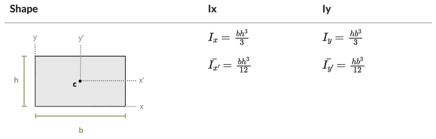
This text uses common shapes or a composite of common shapes for cross-sections. The location of the centroid of some common shapes can be found in Appendix E, part of which is reproduced in Figure 8.3. Each row of the table includes a common shape with the centroid marked and provides simple formulas for determining the centroid’s x and y coordinates and calculating the area of the shape.
Often structural sections are combinations of these standard shapes. These types of sections are called composite sections. As long as we know the location of the centroid of each shape in the section, we do not need to use integration to find the location of the section’s overall centroid. We can use Equation 8.1 in conjunction with the table in Appendix E to find the location of the centroid for composite shapes.
Example 8.1, Example 8.2, and Example 8.3 demonstrate the process for determining the centroid coordinates of composite areas.
Example 8.1
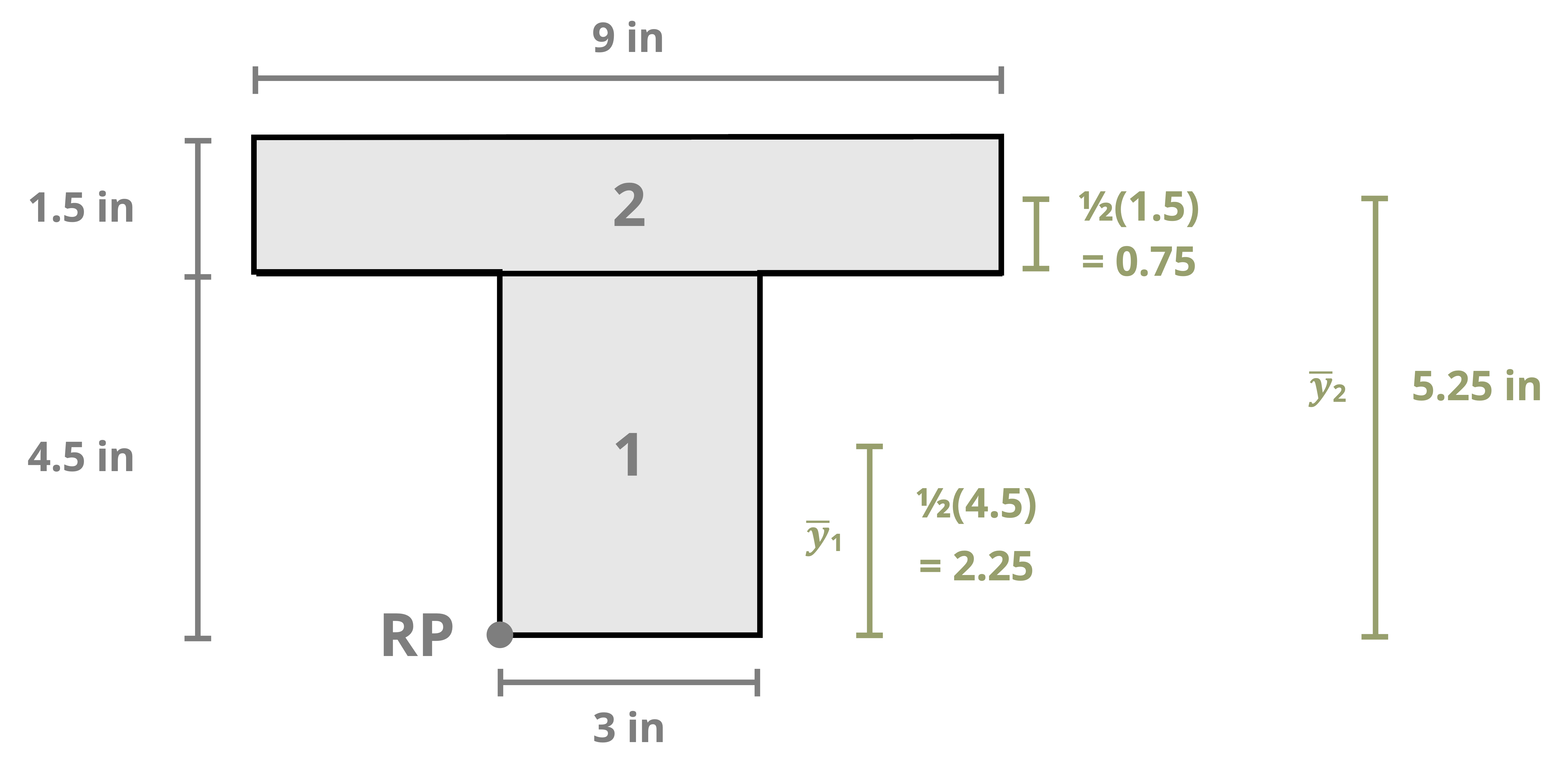
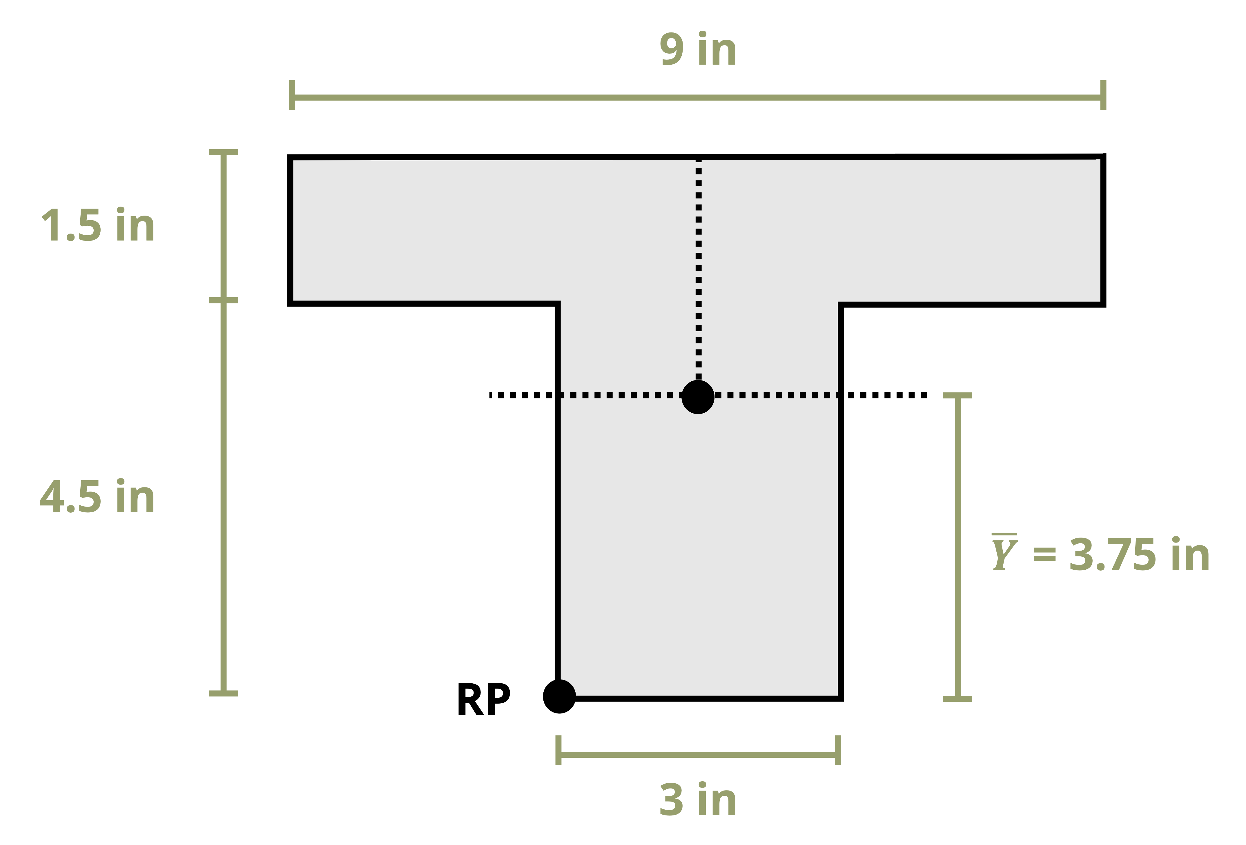
Find the centroid of the shape below.
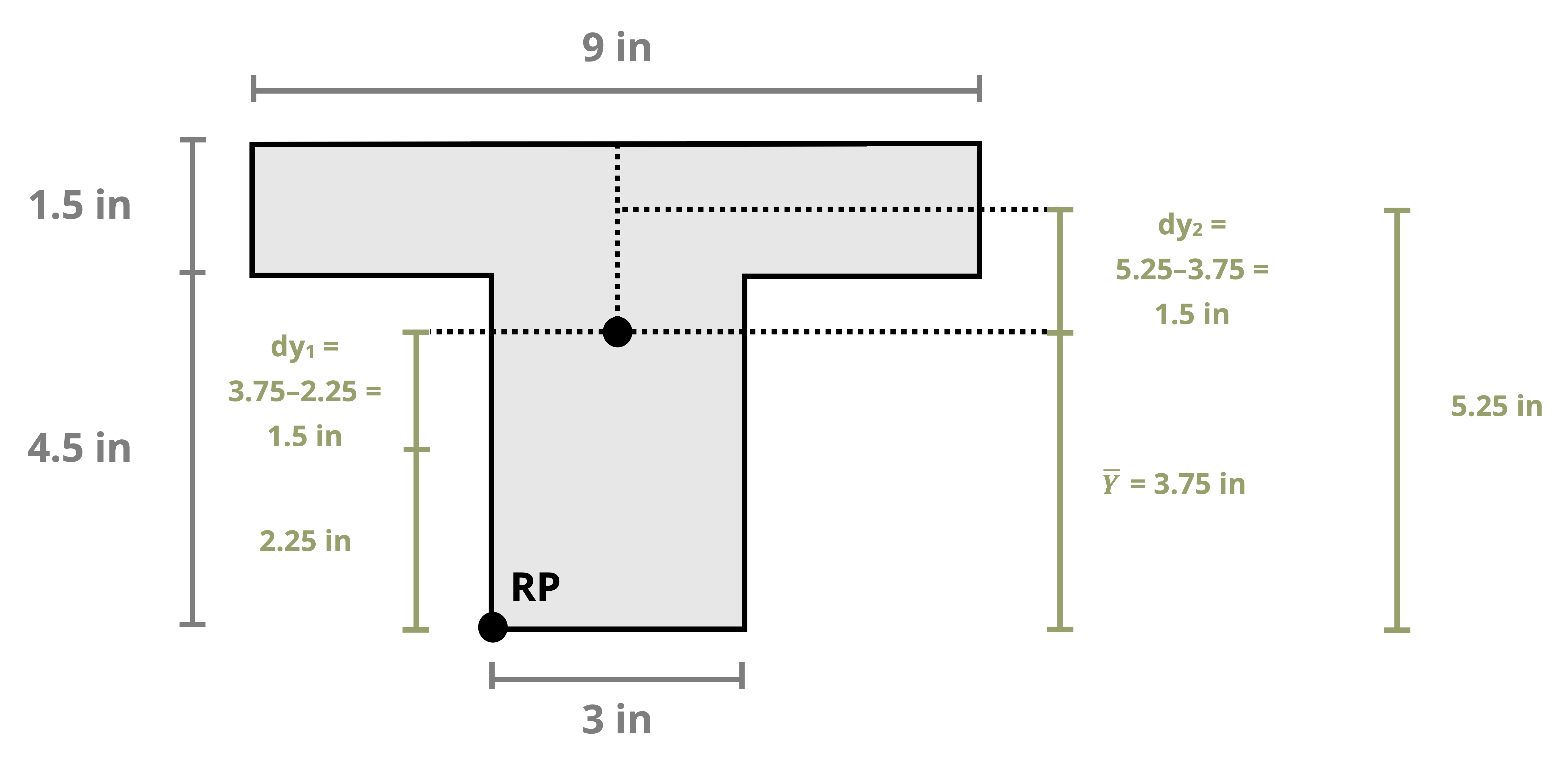
Notice that this T section is symmetric about the y-axis. This means that calculating the centroid in the x direction is unnecessary because we know it will be on that y-axis. We need only find the distance in the y direction, \(\bar{Y}\).
The first thing to do is establish a coordinate system where the origin is the reference point, RP. In this example we chose the bottom left corner of the section so that all y distances will be positive.
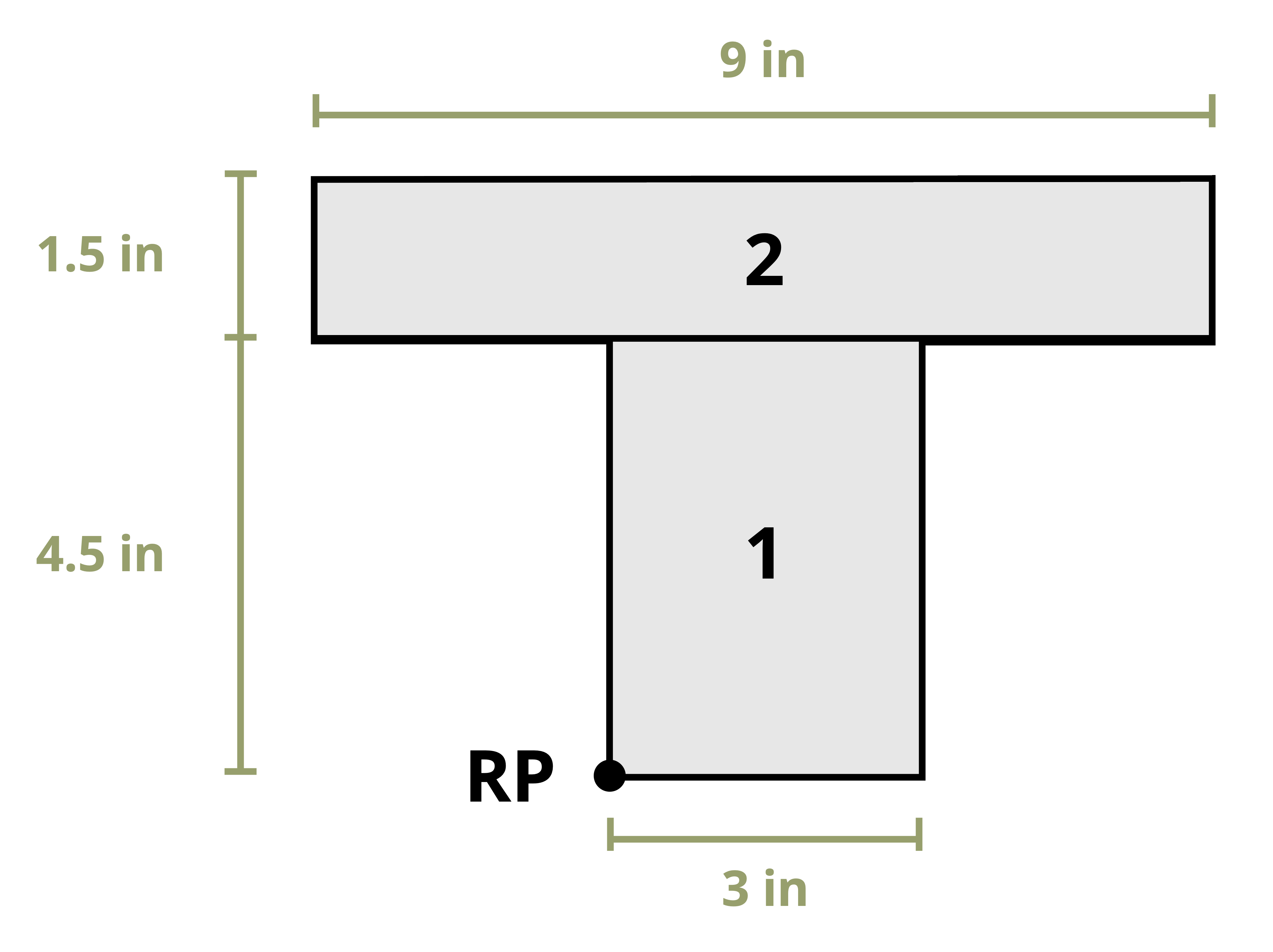
The second step is to divide the section into simpler shapes where we know the location of the centroid. In this case we chose two rectangles, labeled 1 and 2 in the figure.
| Shape | \(A{~(in.^2)}\) | \(\bar{y}{~(in.)}\) | \(A\bar{y}{~(in.^3)}\) |
|---|---|---|---|
| 1 | 13.5 | 2.25 | 30.375 |
| 2 | 13.5 | 5.25 | 70.875 |
| \(\sum A\)=27 | \(\sum A\bar{y}\)=101.25 |
Next is to create a table with columns titled Shape, \(A\) (in.2), \(\bar{y}\) (in.), and \(A\bar{y}\) (in.3). Given two shapes, there will be two rows in the table. Column A is the area of the individual shape. Column \(\bar{y}\) is the perpendicular distance in the y direction from the RP to the centroid of that shape. For example, for shape 1 the \(\bar{y_1}\) would be half of 4.5 in. since the bottom of shape 1 aligns with the RP. However, for shape 2 the \(\bar{y_2}\) would be 4.5 in. plus one half of 1.5 in. This formula ensures measuring from the RP as illustrated here.
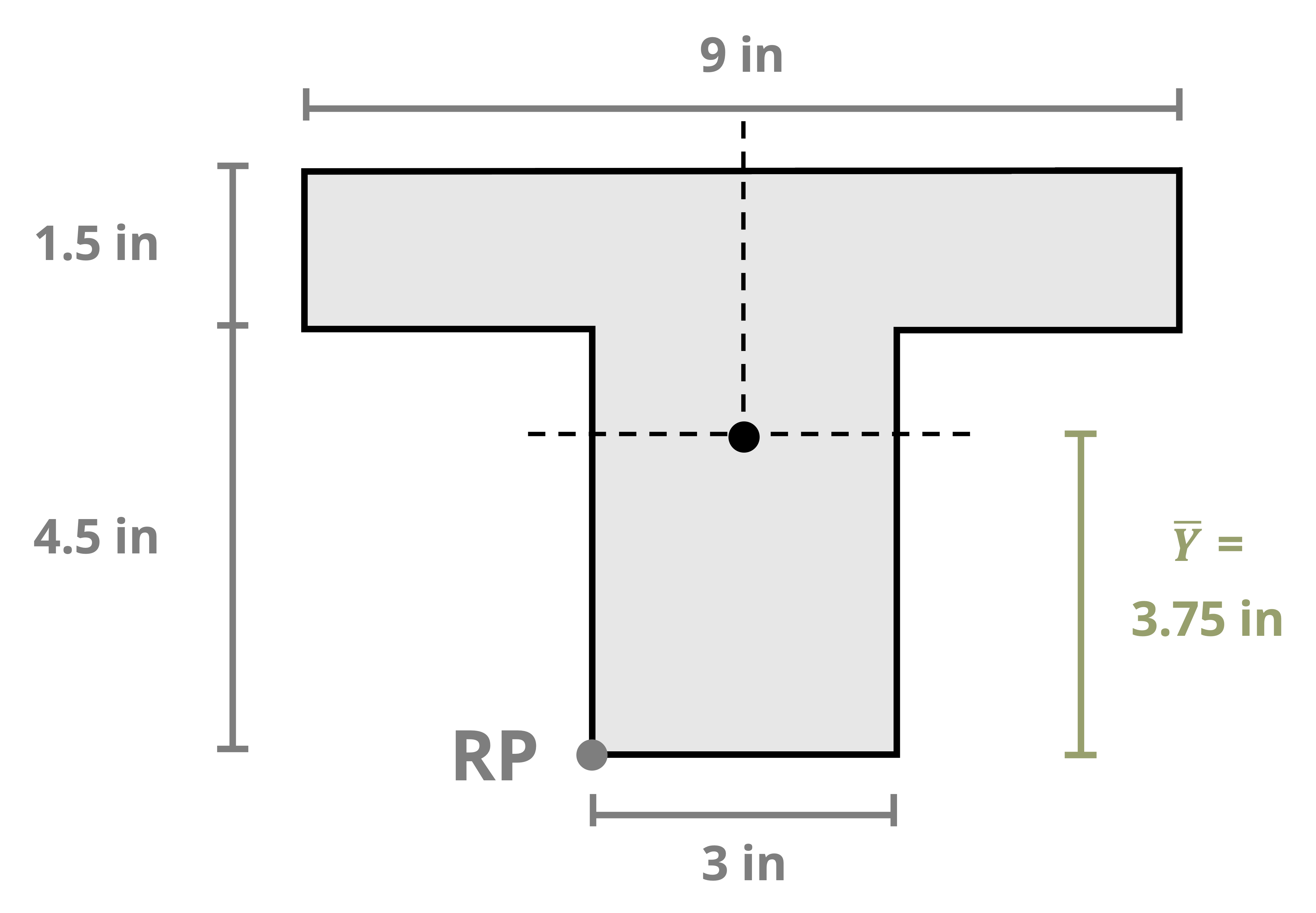
\[ \bar{Y}=\frac{101.25{~in.^3}}{27{~in.^2}}=3.75{~in.} ~~\text{from bottom} \]
Finally, to calculate the centroid coordinates, use Equation 8.1 by summing the last column and the second column in the table. Using this approach we found the centroid to be 3.75 in. from the reference point in the y direction and on the line of symmetry in the x direction.
The following figure shows the location of the centroid for this T section.
Example 8.2
Find the centroid of the illustrated shape.
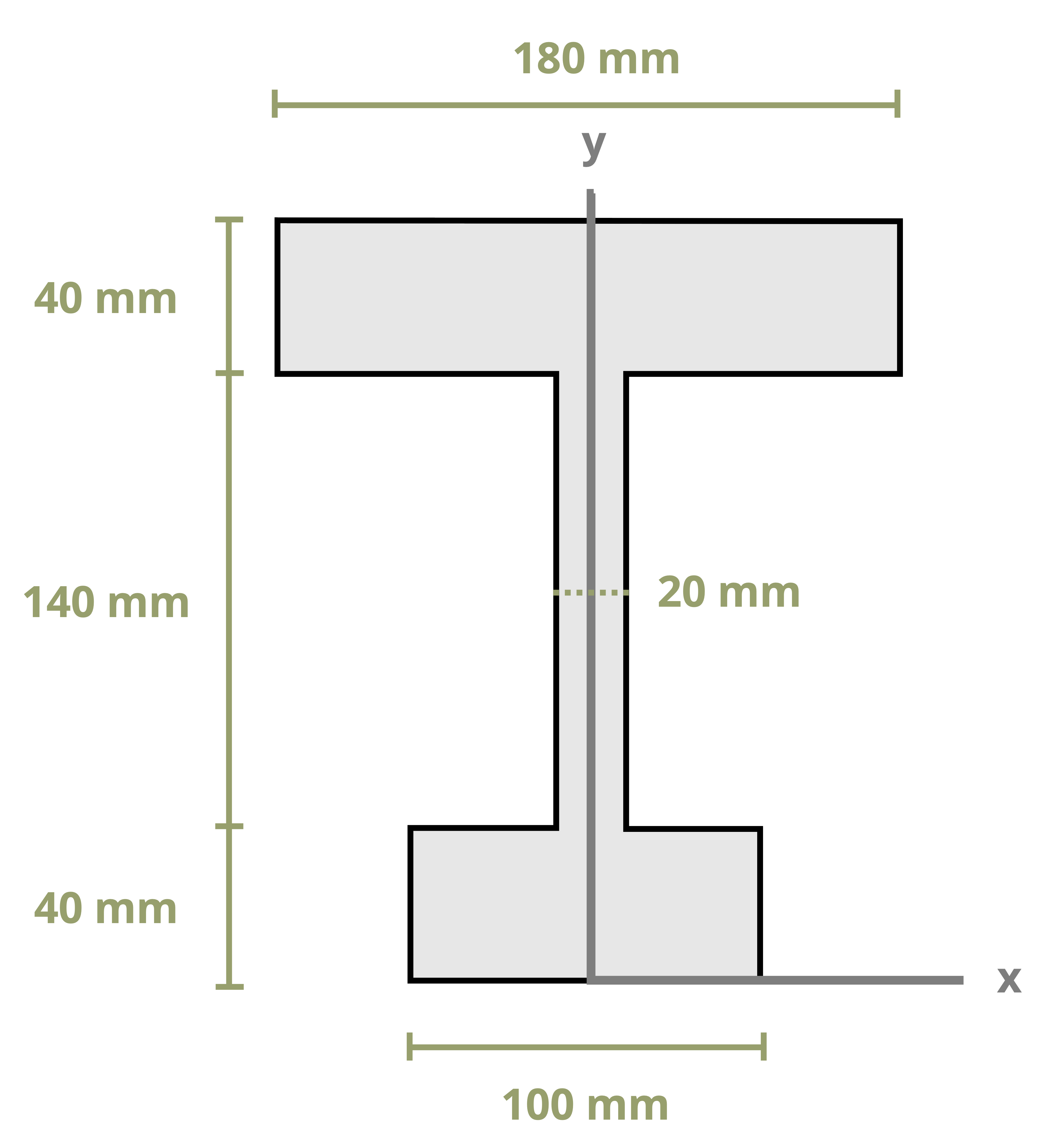
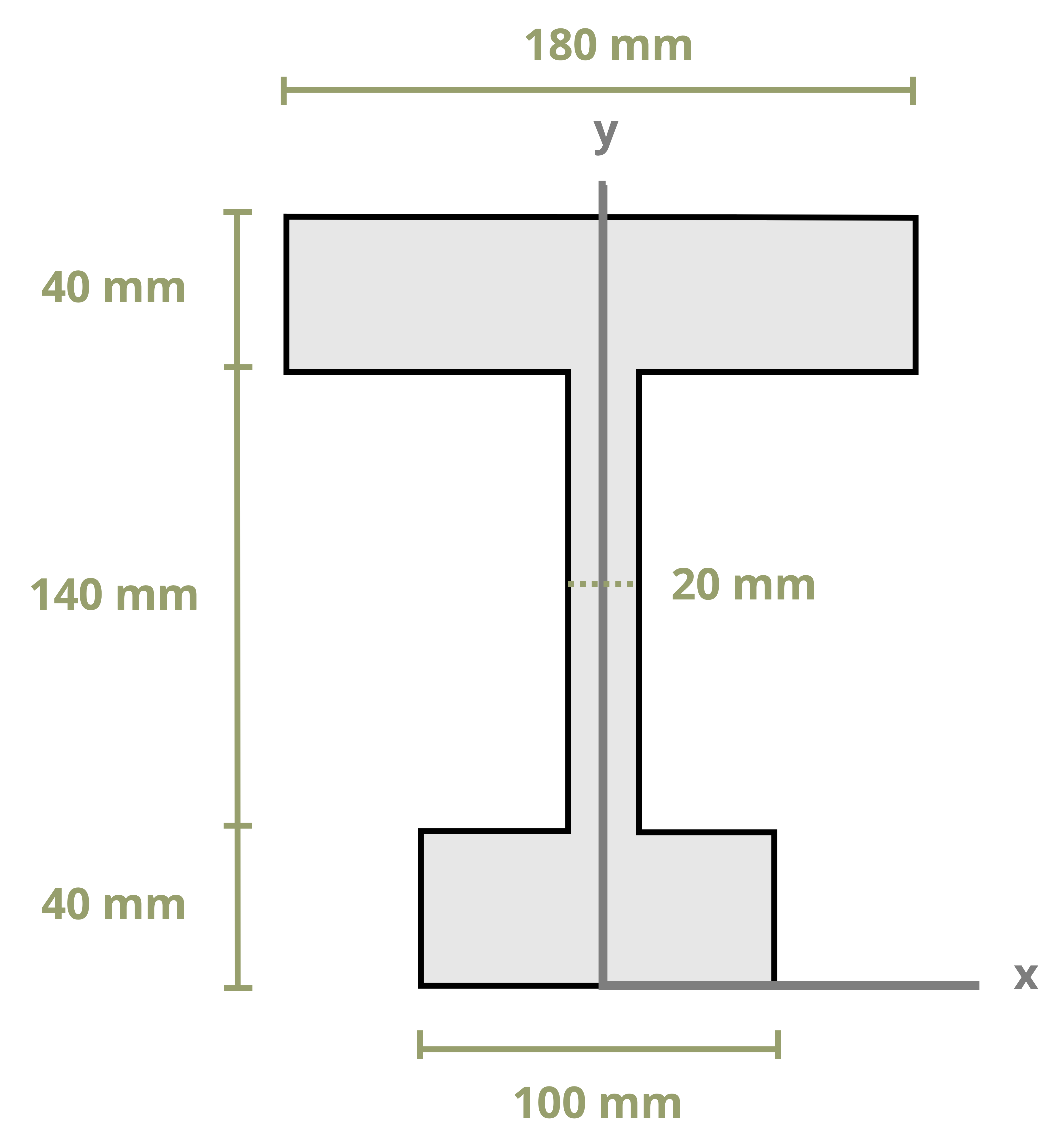
Notice that this section is symmetric about the y-axis, similar to Example 8.1. This means calculating the centroid in the x direction is unnecessary because we know it will be on that y-axis. We need only find the distance in the y direction, \(\bar{Y}\).
The first thing to do is establish a coordinate system whose origin is the reference point, RP. In this example, we chose the bottom of the section along the y-axis so that all y distances will be positive.
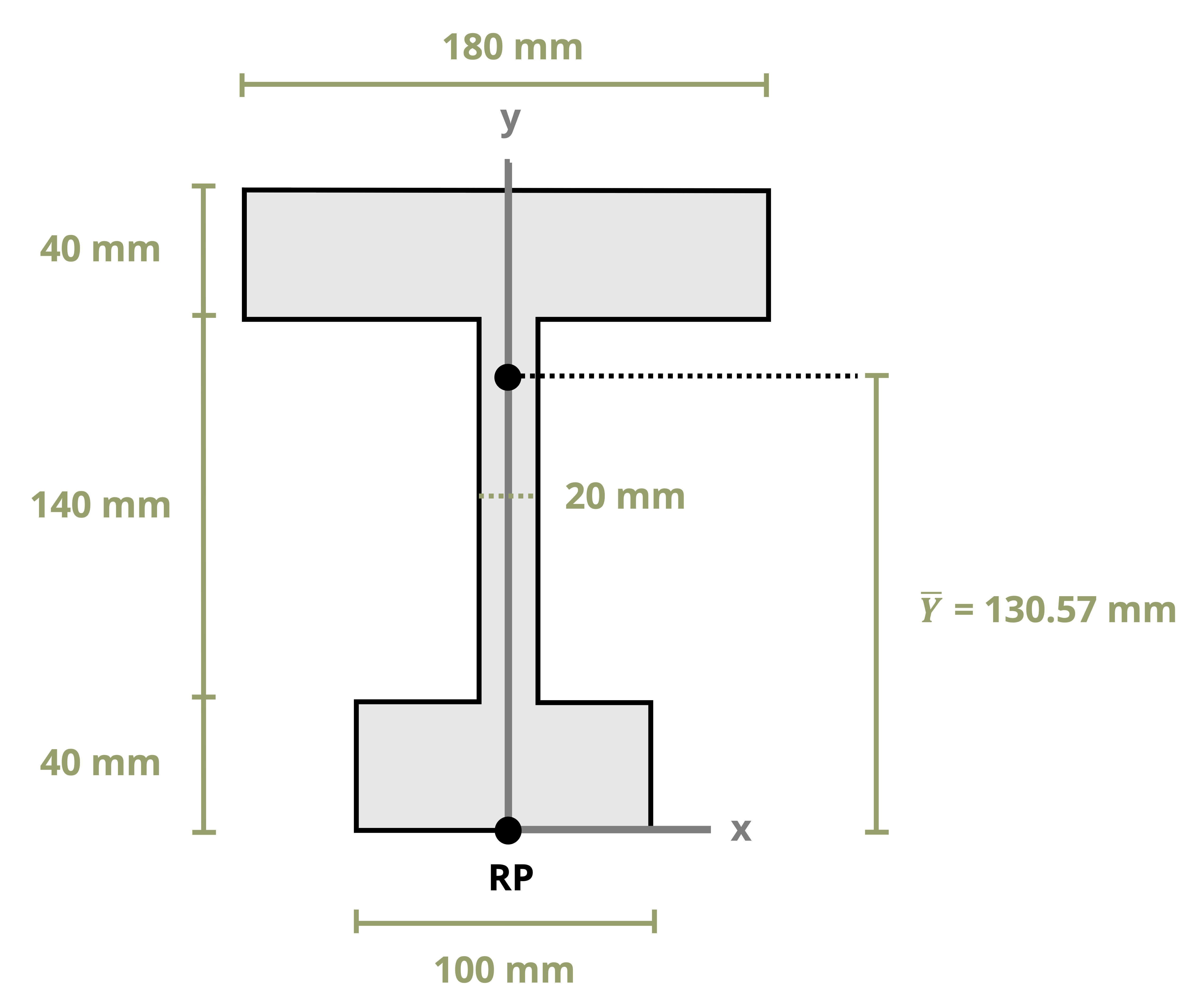
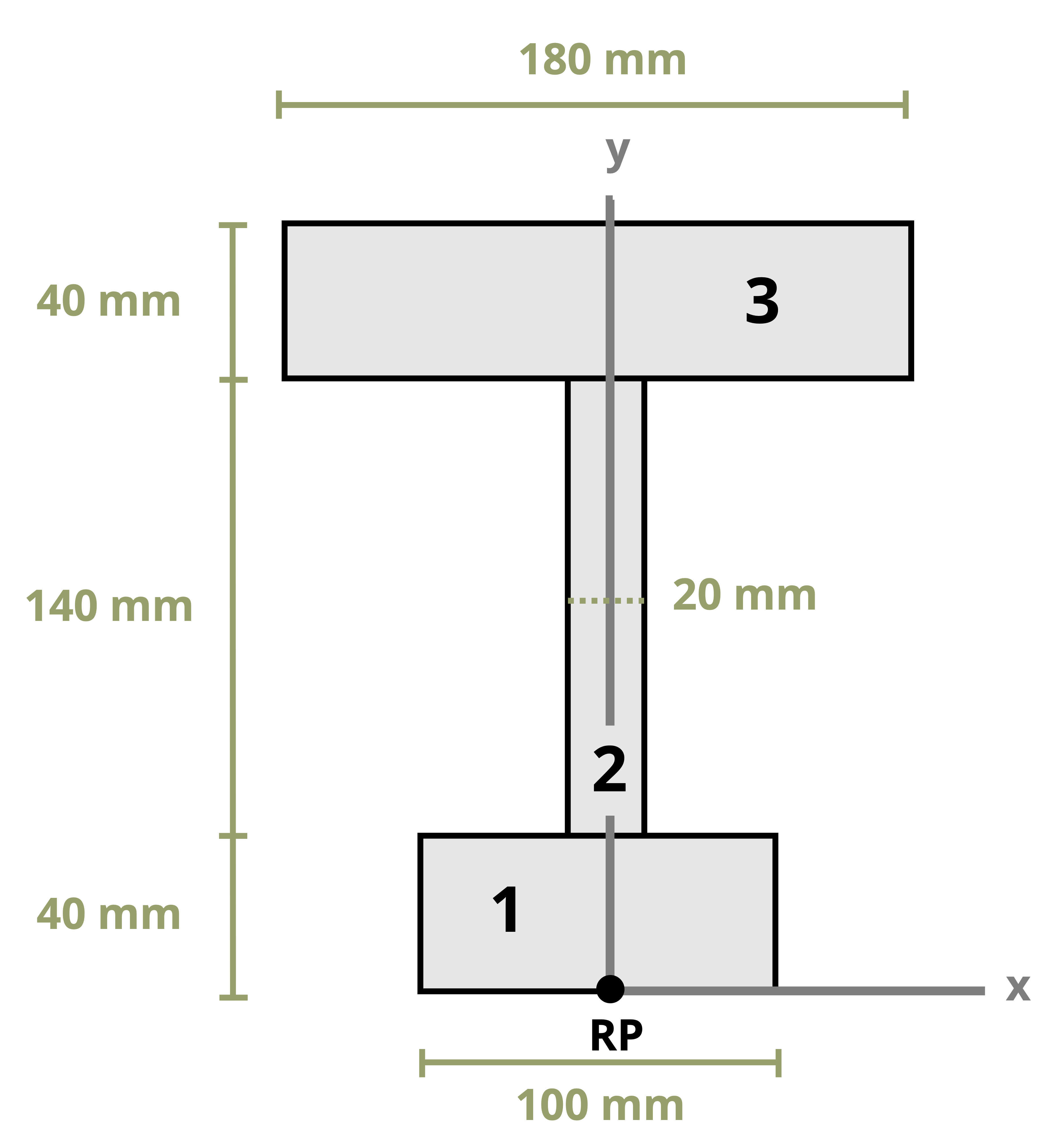
The second task is to divide the section into simpler shapes for which we know the centroid’s location. In this case we chose three rectangles labeled 1, 2, and 3 in the figure.
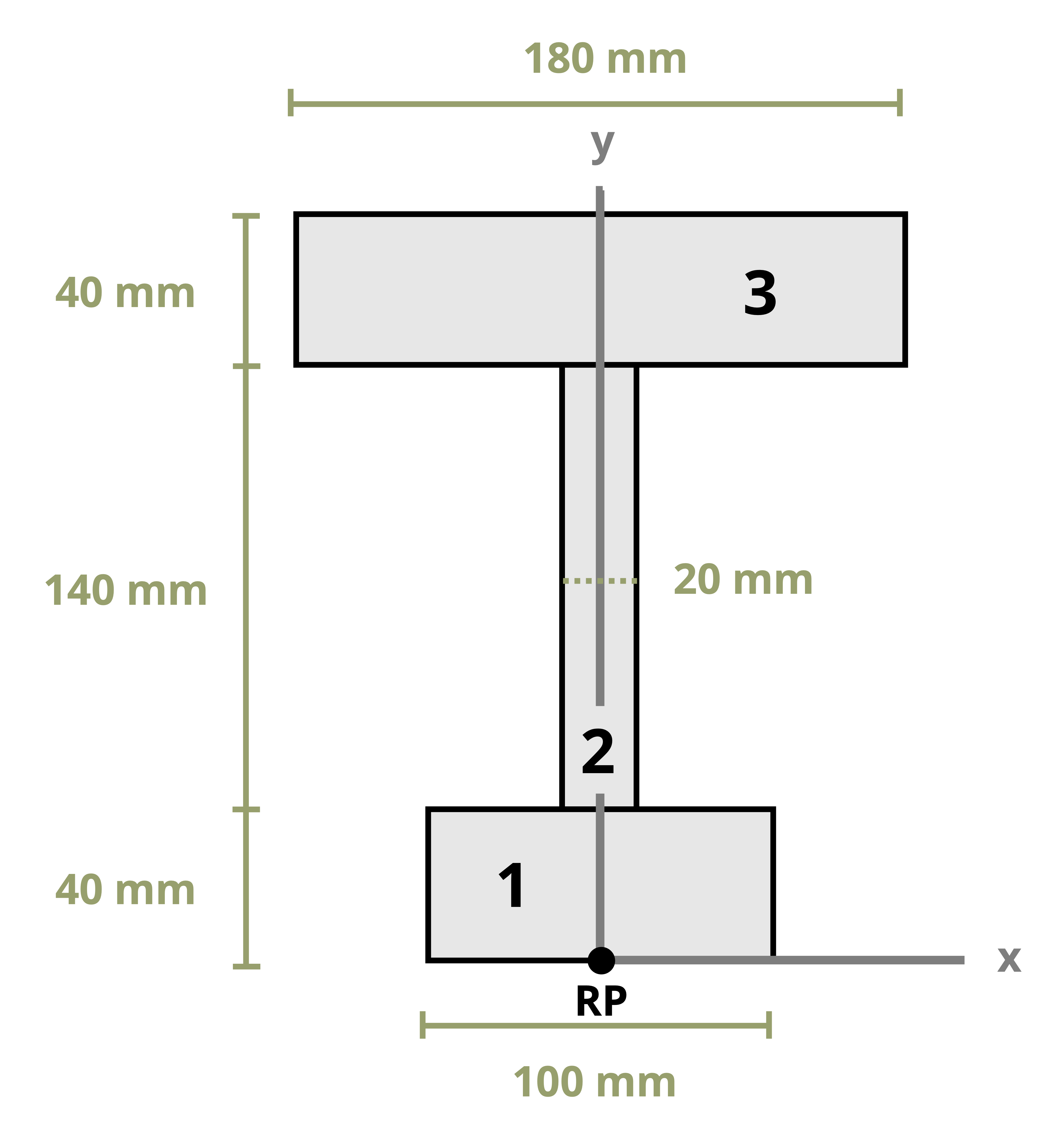
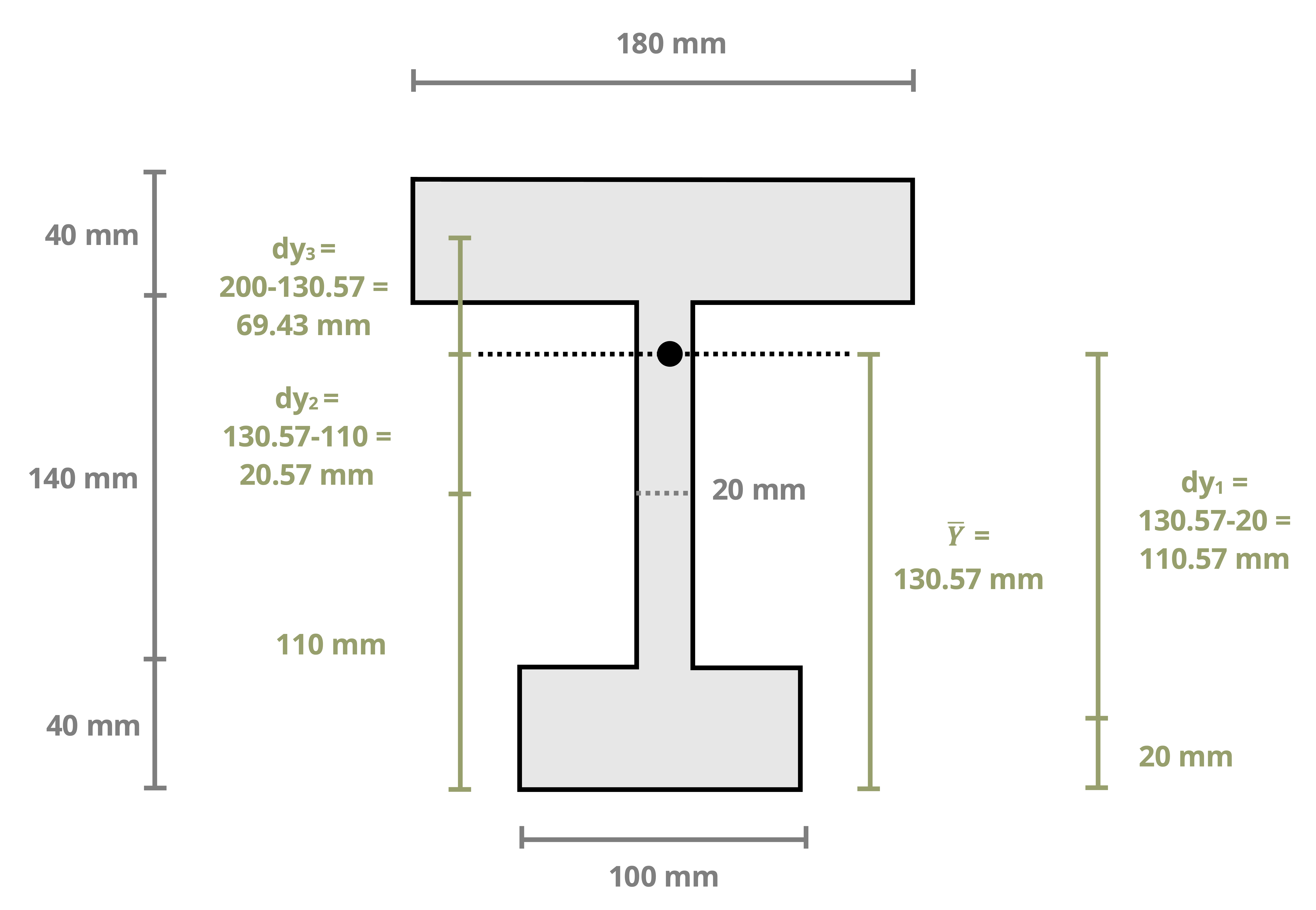
Next, we will create a table with columns titled Shape, \(A\) (mm2), \(\bar{y}\) (mm), and \(A\bar{y}\) (mm3). Given three shapes, there will be three rows. The first column, A, is the area of the individual shape. The second column, \(\bar{y}\), is the perpendicular distance in the y direction from the RP to the centroid of that shape.
The figure below shows how the \(\bar{y}\) for each shape is calculated.
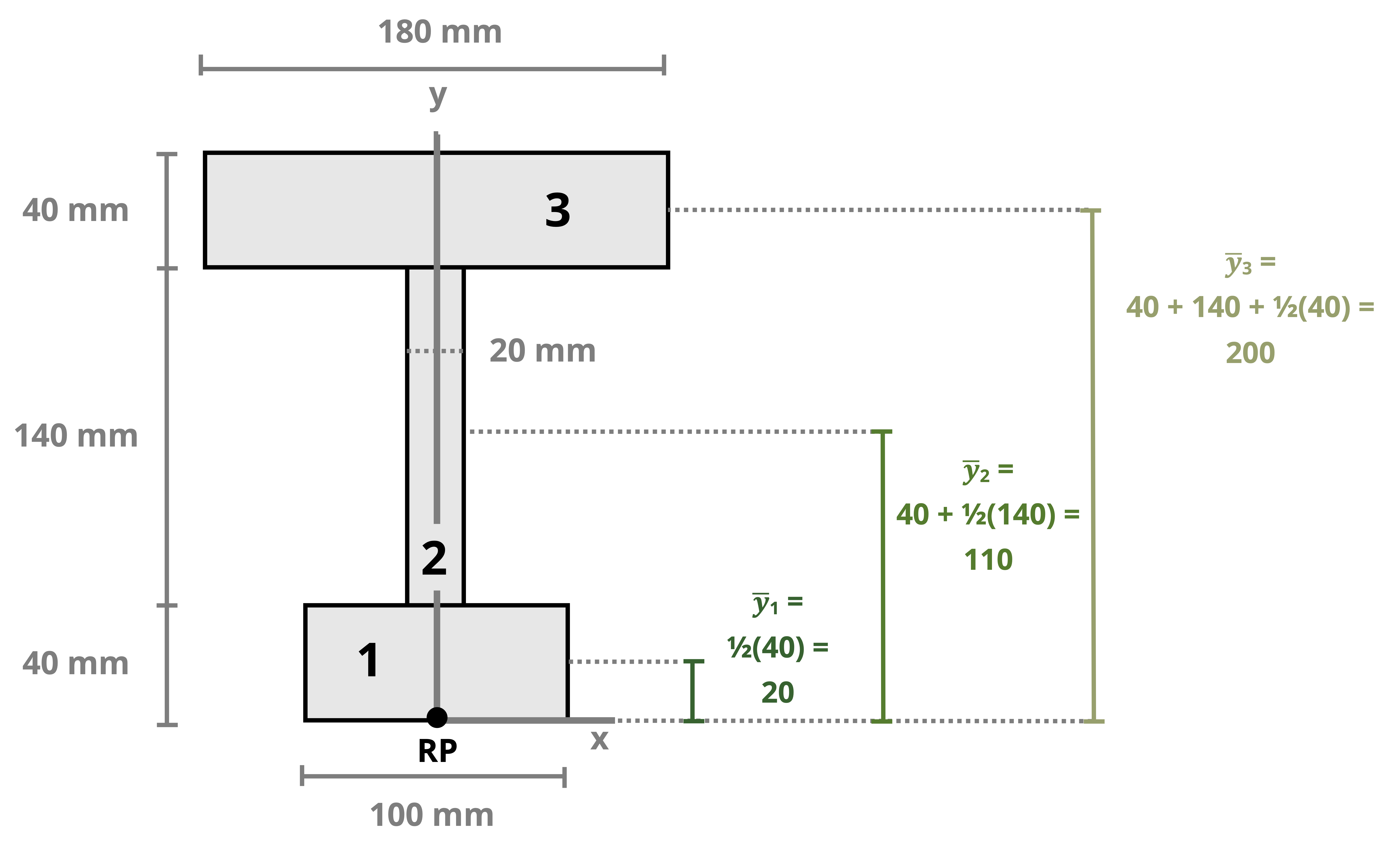
Next is to find the centroid (x̄ = 0 due to symmetry).
| Shape | \(A{~(mm^2)}\) | \(\bar{y}{~(mm)}\) | \(A\bar{y}{~(mm^3)}\) |
|---|---|---|---|
| 1 | 4,000 | 20 | 80,000 |
| 2 | 2,800 | 110 | 308,000 |
| 3 | 7,200 | 200 | 1,440,000 |
| \(\sum A\)=14,000 | \(\sum A\bar{y}\)=1,828,000 |
Finally, to calculate the centroid coordinates, use Equation 8.1 by summing the table’s second and last columns.
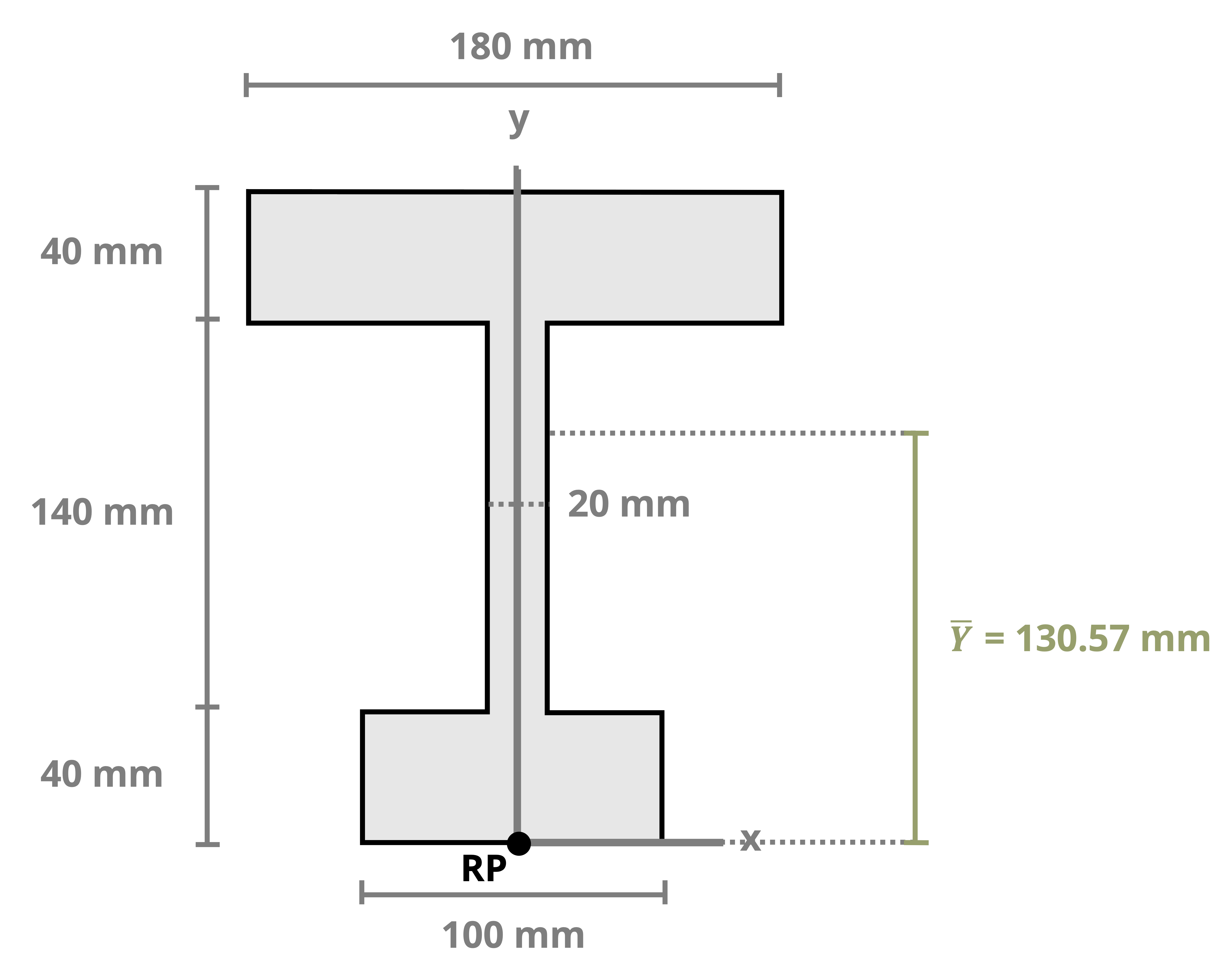
\[ \bar{Y}=\frac{1,828,000{~mm^3}}{14,000{~mm^2}}=130.6{~mm} ~~\text{from bottom} \]
Using this approach we found the centroid to be 130.6 mm from the reference point in the y direction and on the line of symmetry in the x direction.
The figure below shows the location of the centroid for this section.
Example 8.3
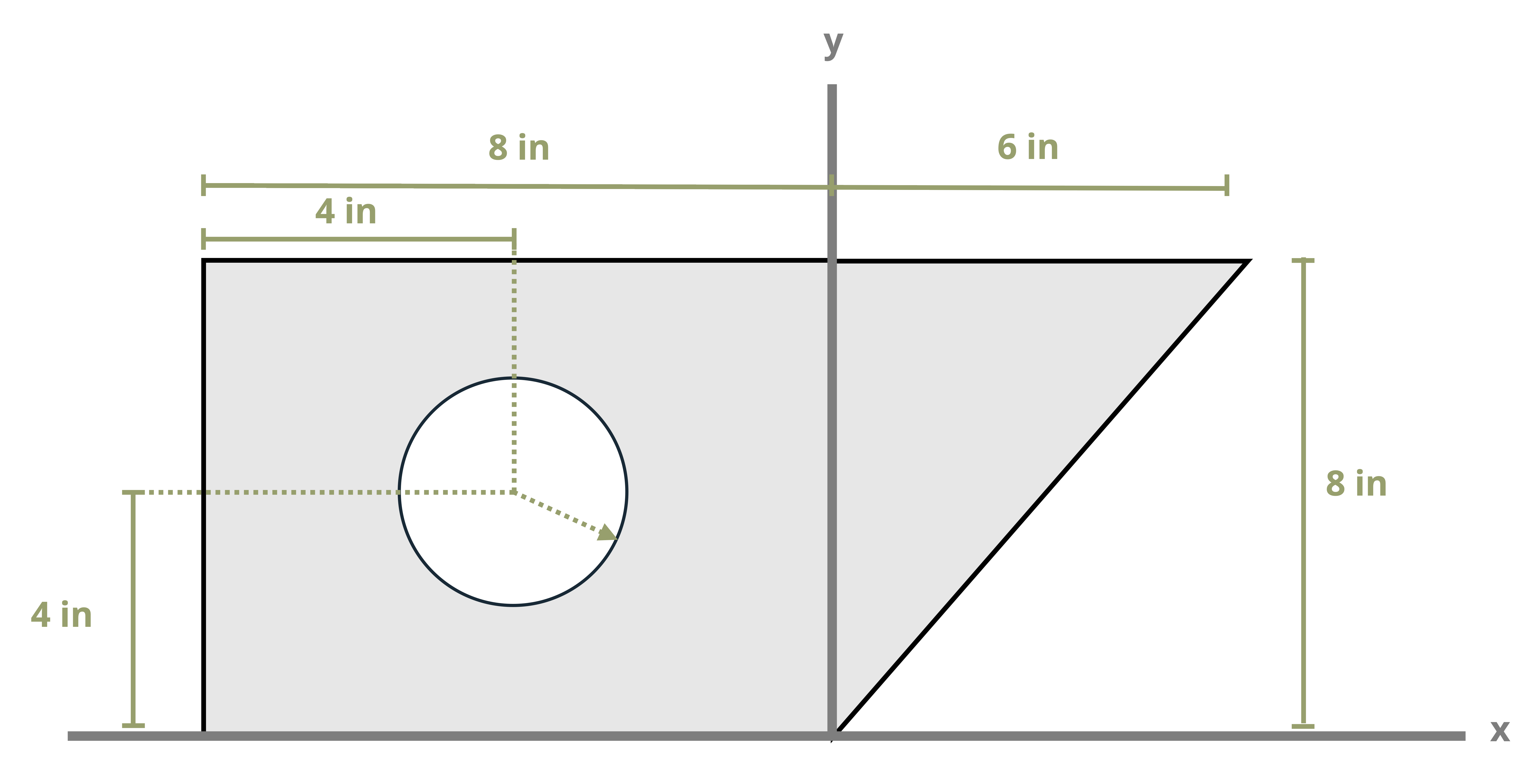
Find the centroid of the shape below.
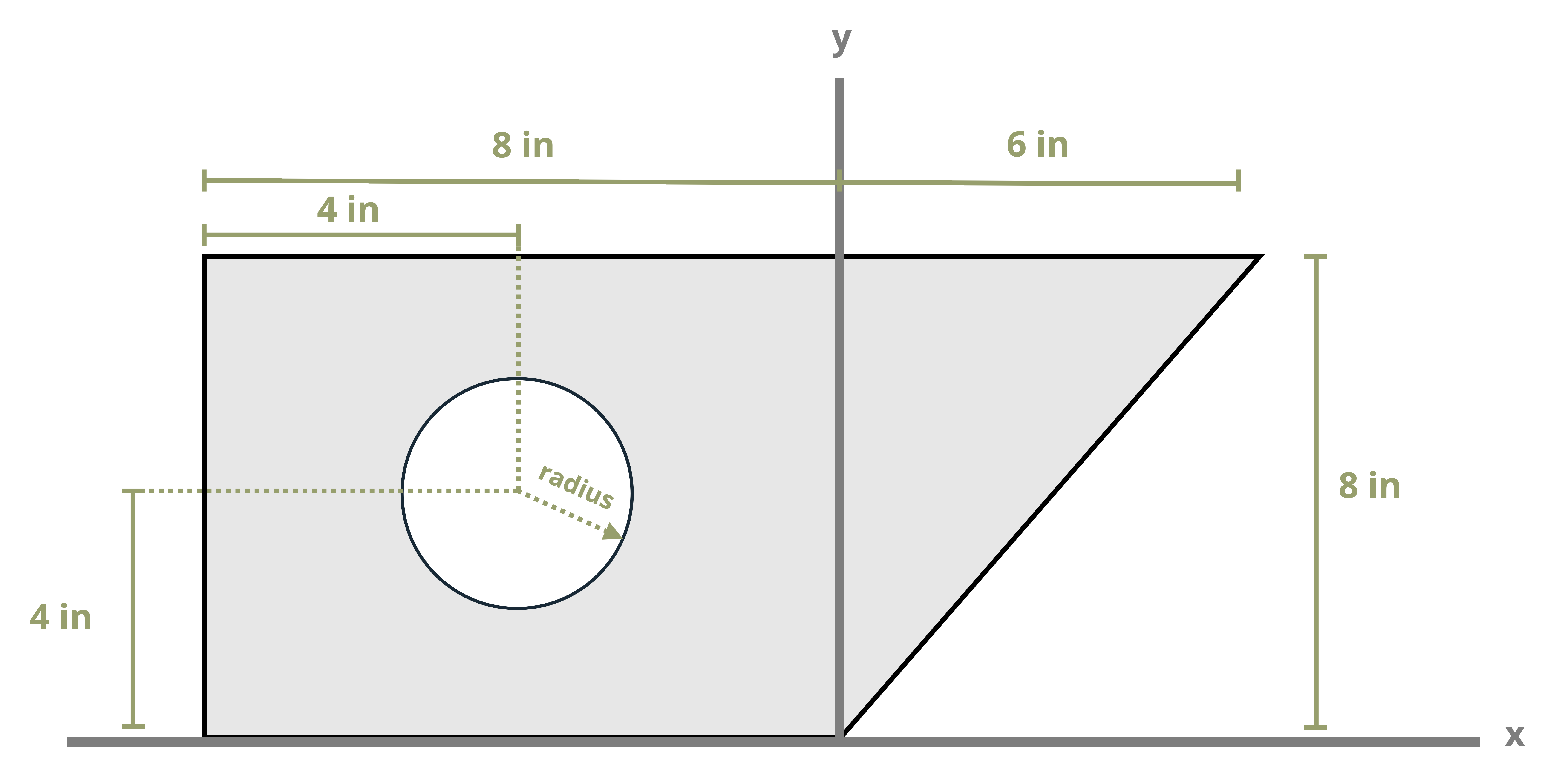
This section has no axis of symmetry, so we must find both the \(\bar{x}\) and the \(\bar{y}\). The first task is to establish a coordinate system whose origin is the reference point, RP. In this example, the coordinate axis in the problem illustrates when \(\bar{x}\) will be negative.
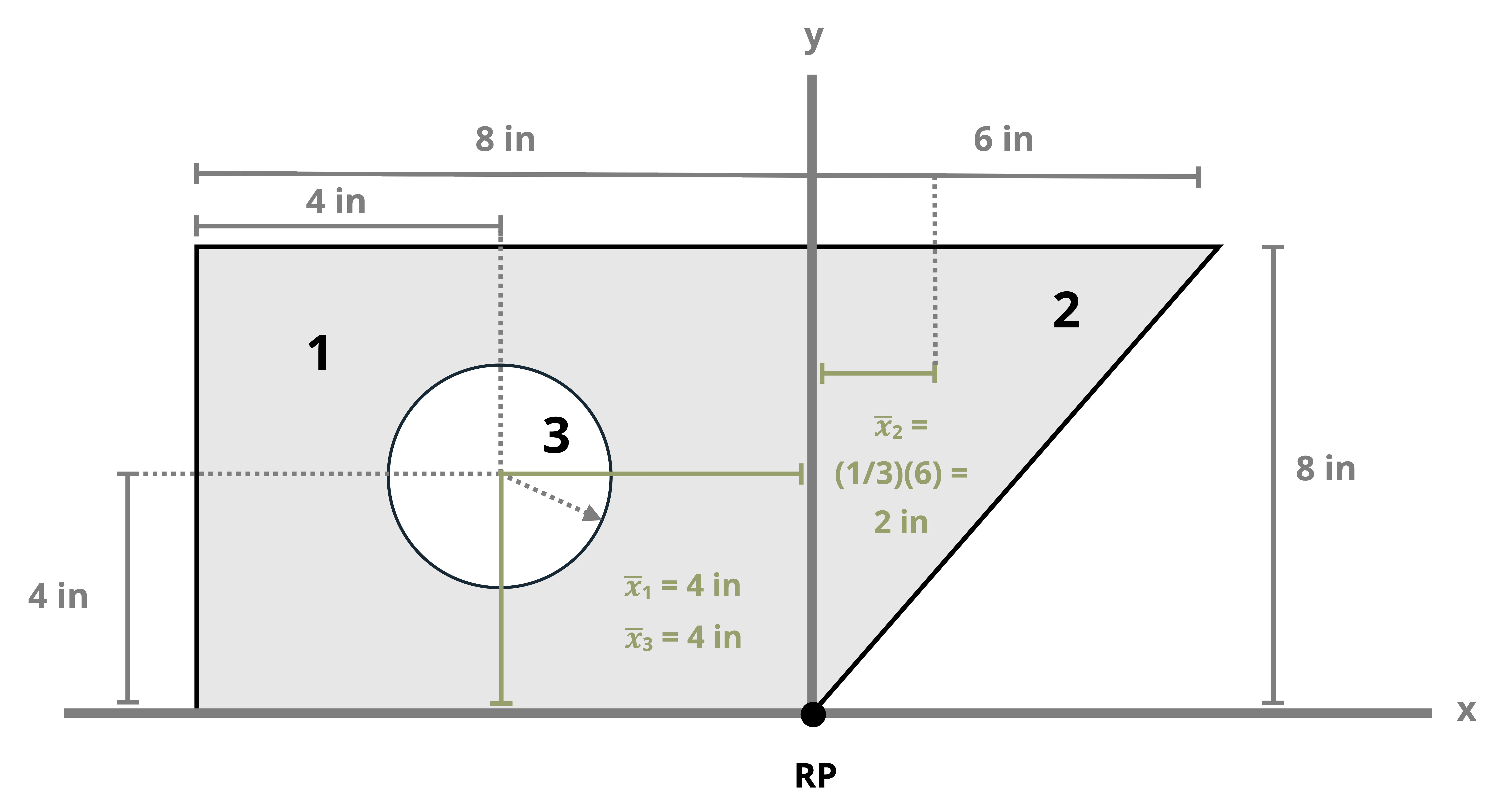
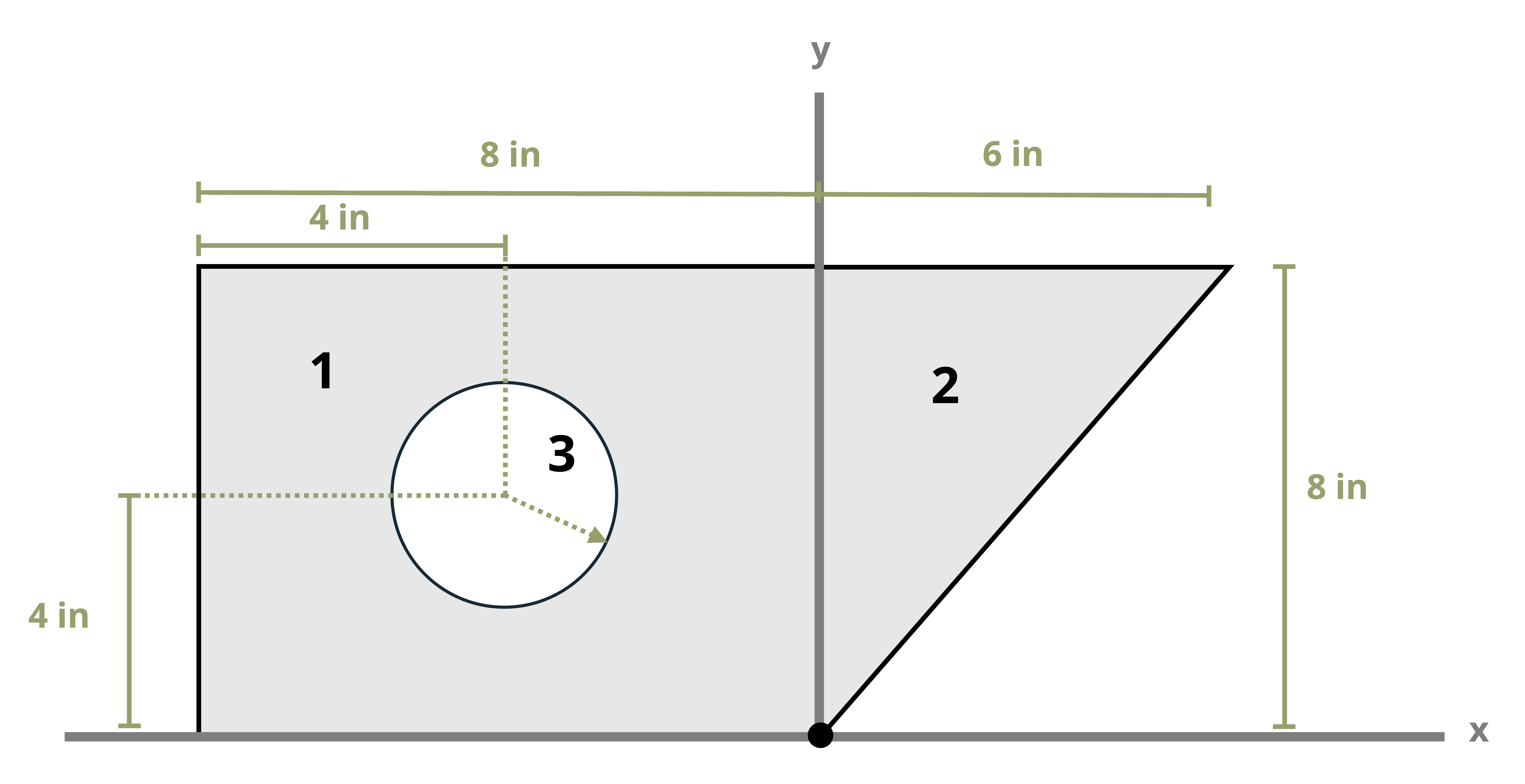
The second task is to divide the section into simpler shapes for which we know the centroid’s location (Appendix E). In this case we will break this up into the square, triangle, and circle labeled 1, 2, and 3 in the figure. Note that the circle is a hole and the area will be represented as negative.
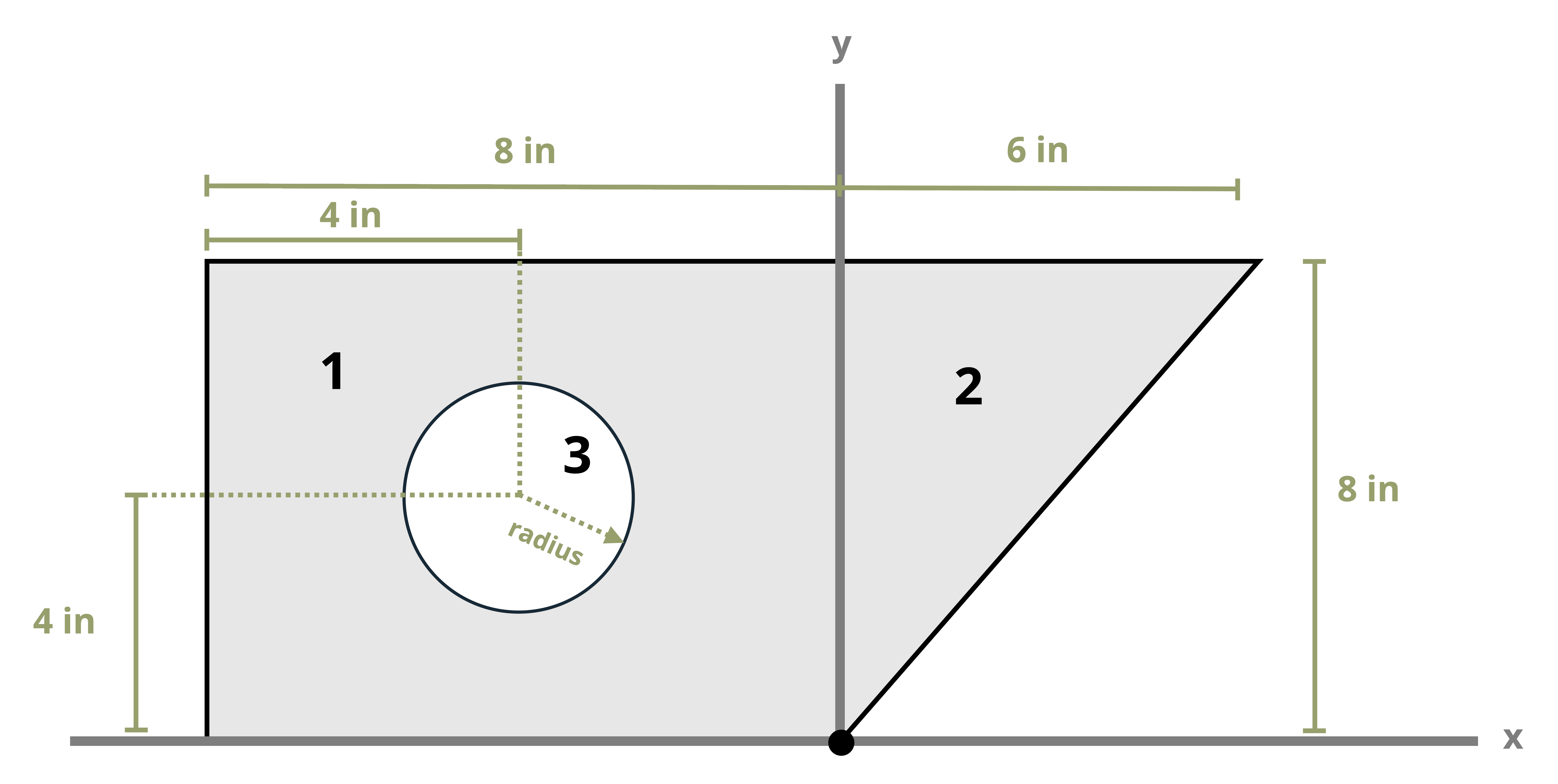
Next is to create a table with columns titled Shape, \(A\) (in2), \(\bar{x}\) (in), \(\bar{y}\) (in), and \(A\bar{y}\) (in3). Given three shapes, there are three rows. The first column, A, is the area of the individual shape. The second column, \(\bar{x}\), is the perpendicular distance in the x direction from the RP to the centroid of that shape.
The figure below shows how the \(\bar{x}\) for each shape is calculated.
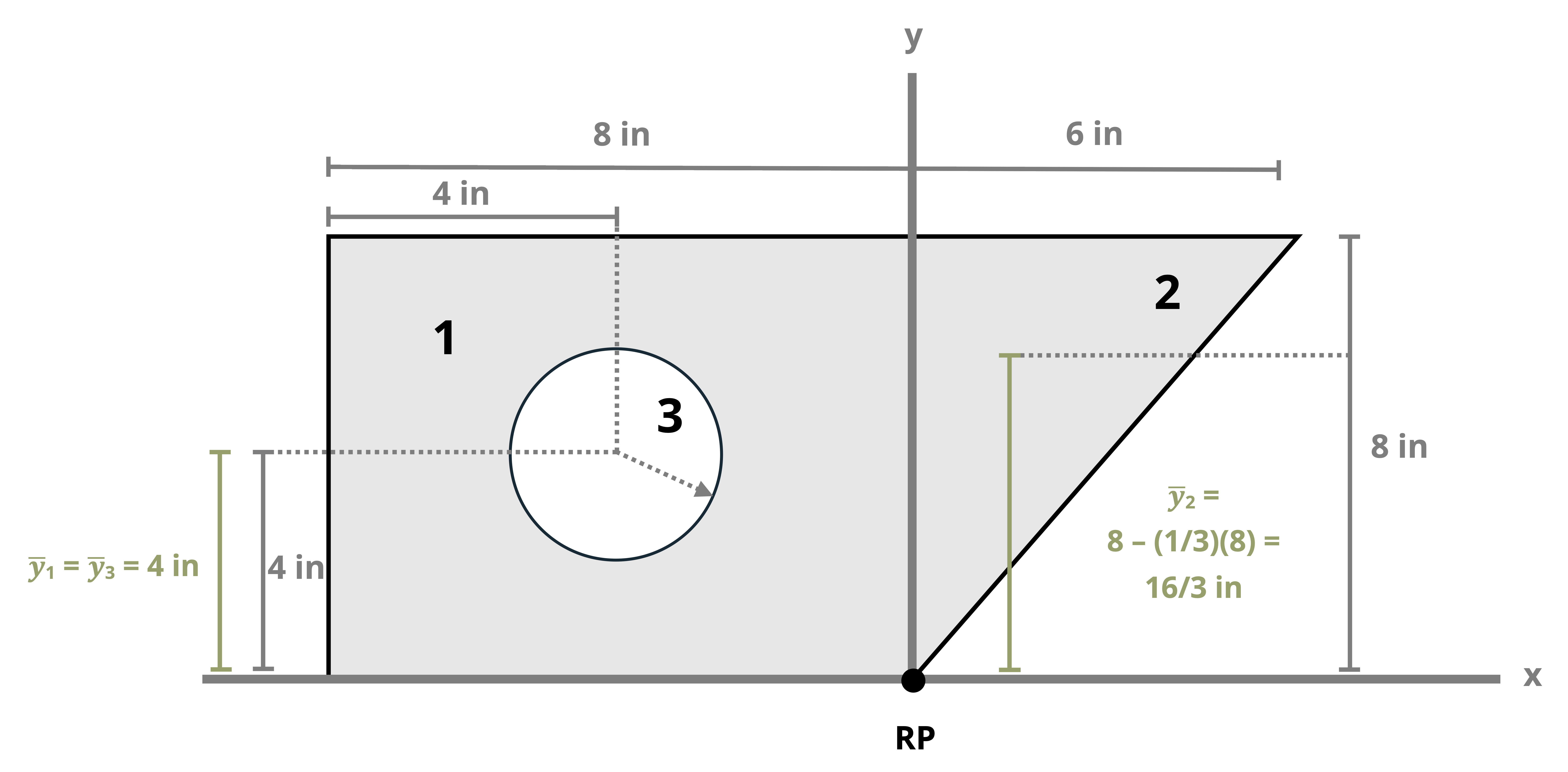
The figure below shows how the \(\bar{y}\) for each shape is calculated.
Finally, to calculate the centroid coordinates, use Equation 8.1 by summing the A, \(A\bar{x}\), and \(A\bar{y}\) columns shown in the table below.
| Shape | \(A{~(in.^2)}\) | \(\bar{x}{~(in.)}\) | \(A\bar{x}{~(in.^3)}\) | \(\bar{y}{~(in.)}\) | \(A\bar{y}{~(in.^3)}\) |
| 1 | 64 | -4 | -256 | 4 | 256 |
| 2 | 24 | 2 | 48 | (2/3)(8) = 16/3 | 128 |
| 3 | -4π | -4 | 16π | 4 | -16π |
| \(\sum A\) = 75.4 | \(\sum A\bar{x}\)= -258.3 | \(\sum A\bar{y}\)= 333.7 |
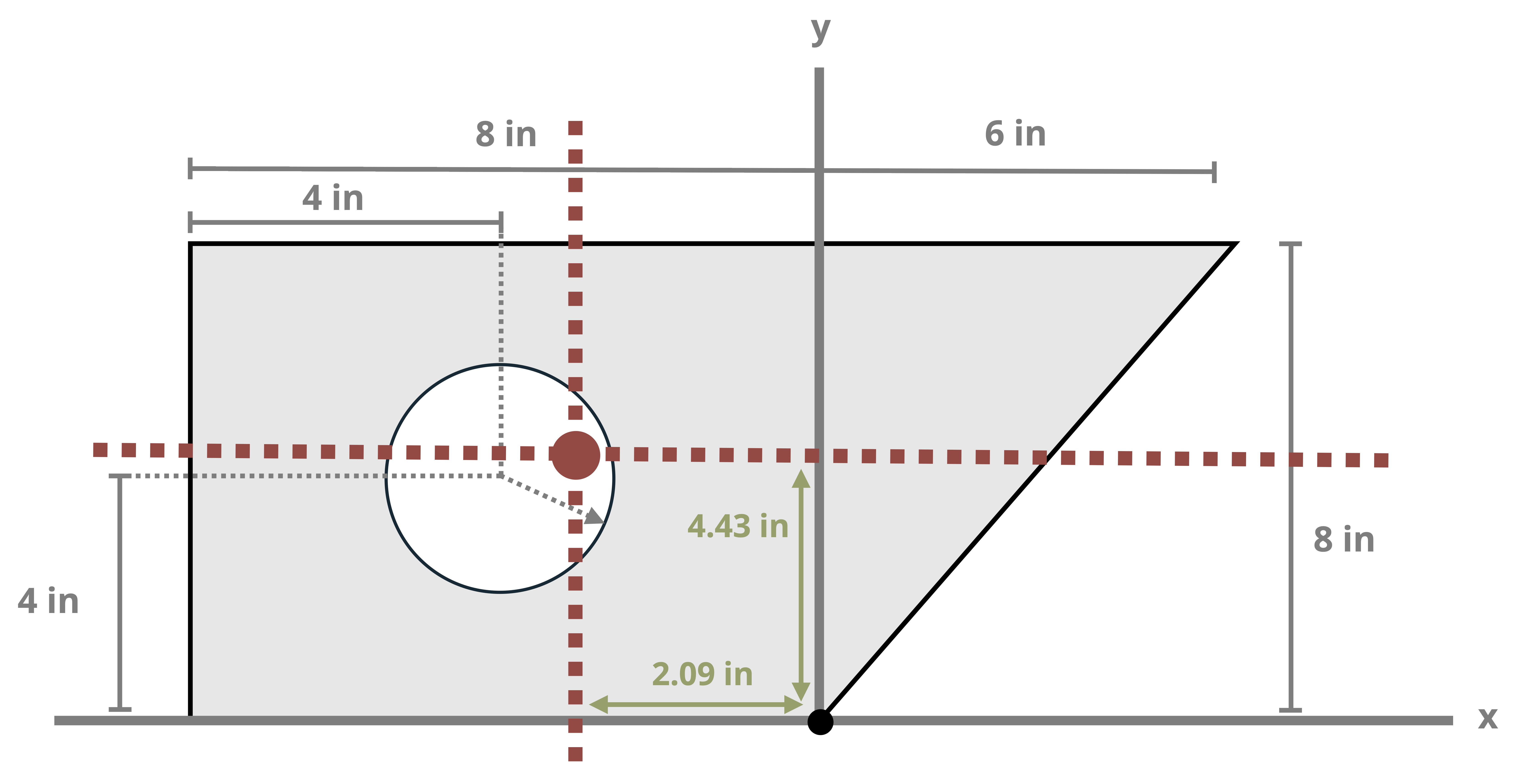
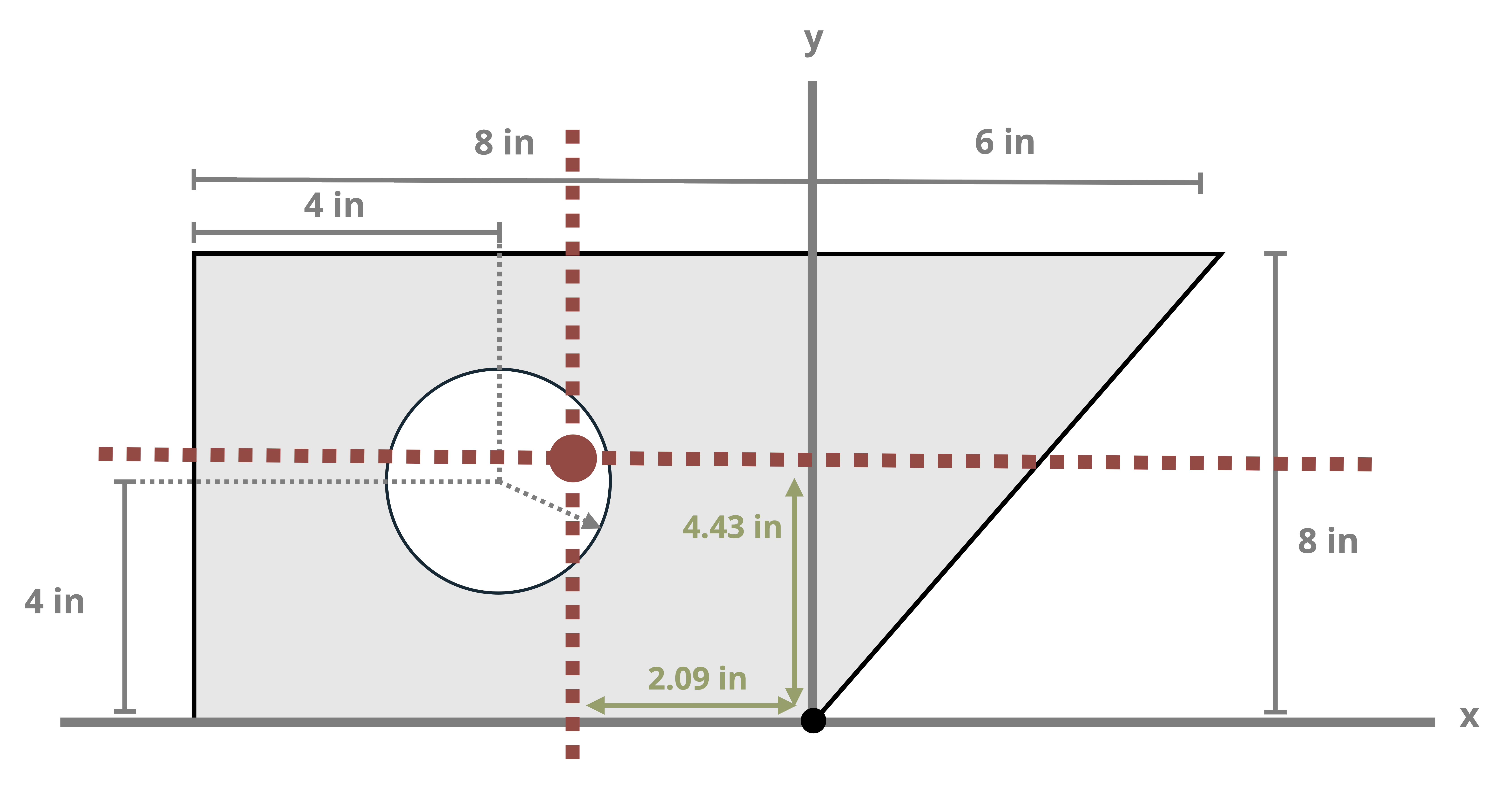
\[ \begin{aligned} & \bar{X}=\frac{\sum A \bar{x}}{\sum A}=\frac{-157.7{~in.^3}}{75.4{~in.^2}} \quad\rightarrow\quad \bar{X}=-2.09{~in} \\ & \bar{Y}=\frac{\sum A \bar{y}}{\sum A}=\frac{333.7{~in.^3}}{75.4{~in.^2}} \quad\rightarrow\quad \bar{Y}=4.43 \mathrm{in} \end{aligned} \]
Using this approach, we calculated the centroid to be -2.09 in. in the x direction from the reference point, which indicates it will be to the left of the y-axis. The y component of the centroid is 4.43 in. in the y direction from the reference point.
The figure below shows the location of the centroid for this section.
8.2 Second Moment of Area
Click to expand
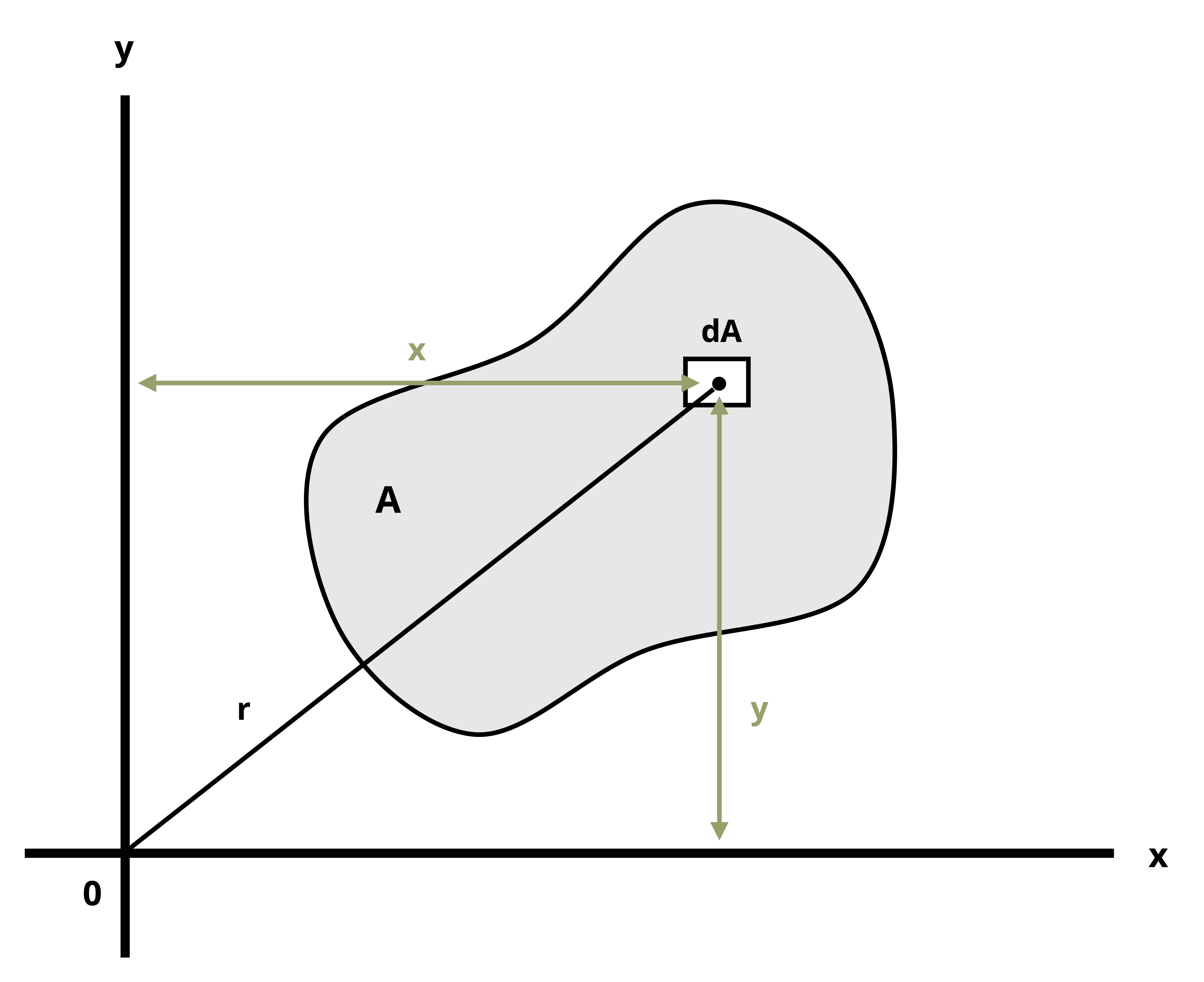
Another important geometric property needed to calculate stresses in beams is the second moment of area (also known as moment of inertia and area moment of inertia). You likely encountered this topic in statics, as you did the topic of centroids, so this section is designed as a review. By definition the second moment of area depicted in Figure 8.4 is
\[ \boxed{\begin{aligned} &I_x=\int_A y^2 d A \\ &I_y=\int_A x^2 d A \\ &I_z=J=\int_A r^2 d A \\ \end{aligned}} \tag{8.2}\]
Keep in mind that this text uses common shapes or a composite of common shapes for cross-sections. Appendix E includes formulas to calculate the second moment of area. Part of Appendix E is reproduced in Figure 8.5. Each row of the table includes a common shape with the centroid marked and with formulas for determining the second moment of area about the centroidal axes x, y, and z. Note that these equations are valid only for the axes passing through the area’s centroid and are written as \(\overline{I_{x^{\prime}}}\), \(\overline{I_{y^{\prime}}}\), and J respectively. The bar notation is used to signify that the second moment of area is being calculated around the centroidal axes.
As noted previously, structural sections, called composite sections, are often combinations of these standard shapes. As with calculating centroids, we break these composite sections into common shapes and find the second moment of area of these individual shapes. When calculating each individual shape’s second moment of area, we must ensure that they are all about the same axis.
The parallel axis theorem provides a method for calculating the second moment of area about an axis parallel to an axis passing through the centroid, given that the second moment of area about the latter axis is known.
To establish the parallel axis theorem, we’ll next examine the second moment of area about A relative to an axis x, as illustrated in Figure 8.6.
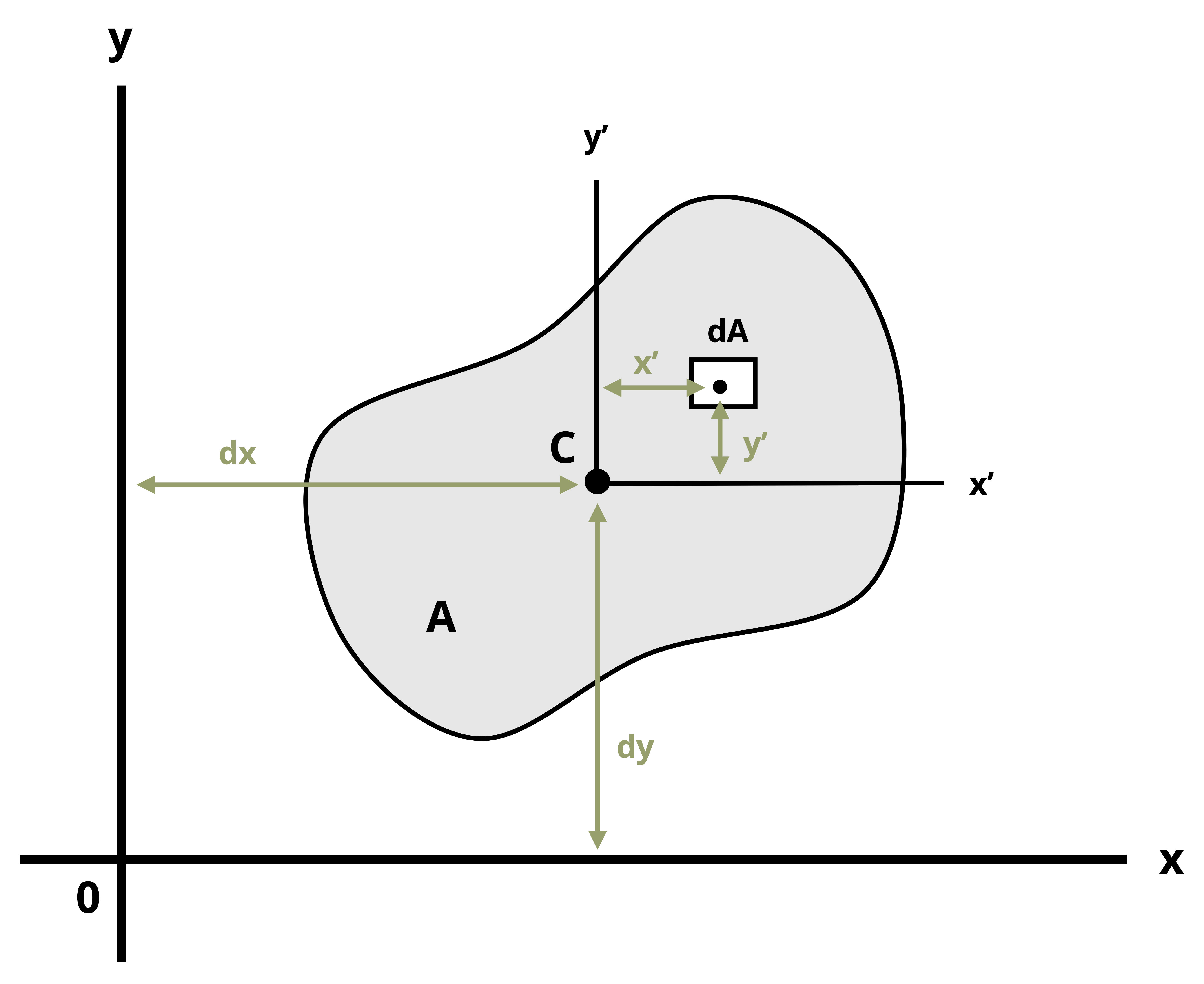
The centroid of the area is at C, where the x’-y’ axis is drawn; note that x’ is parallel to x and y’ is parallel to y. The x-y’ axes will be termed the centroidal axes and are at a distance of dx and dy from the x-y axes respectively. The distance between the element dA and the x’-axis is denoted as y’. The result is \(y=y^{\prime}+d_y\). Substituting into Equation 8.2 yields
\[ \begin{aligned} & I_x=\int\left(y^{\prime}+d_y\right)^2 d A \\ & I_x=\int\left(y^{\prime}\right)^2 d A+2 d_y \int y^{\prime} d A+d_y^2 \int d A \end{aligned}\text{ .} \]
The first integral represents the second moment of area about the centroidal axis x’. The second integral is zero since the centroid is located on the x’-axis (i.e., \(\int y^{\prime} d A\) represents the first moment of area about the x’ centroidal axis, which is zero, as discussed in Section 8.1). The last integral represents the total area, A. So the resulting equation is
\[ \boxed{I_x=\overline{I_{x^{\prime}}}+A d_y^2}\text{ .} \tag{8.3}\]
A similar process is used to find an expression for Iy.
\[ \boxed{I_y=\overline{I_{y^{\prime}}}+A d_x^2}\text{ ,} \tag{8.4}\]
Ix, Iy = Second moment of area with respect to a given axis [m4, in.4]
\(\overline{I_{x^{\prime}}}\) , \(\overline{I_{y^{\prime}}}\) = Second moment of area with respect to a parallel axis passing through the centroid of the area [m4, in.4]
A = Area [m2, in.2]
dx, dy = Perpendicular distance between the given axis and the parallel centroidal axis [m, in.]
While the parallel axis theorem can be used to calculate the second moment of area around any pair of axes, here the focus is primarily on calculating the second moment of area around the centroidal axes of a composite region (this is this term used in Chapter 9 and Chapter 10 when calculating bending stresses and shear stresses). Example 8.4, Example 8.5, and Example 8.6 demonstrate using the parallel axis theorem to find the second moment of area for the composite areas from the earlier examples about their centroidal axes.
Example 8.4
Determine the Ix of the shaded area with respect to the section’s centroid.

To find the second moment of area in the x direction with respect to the section’s centroid, first calculate the centroid. We did this in Example 8.1, with the results as shown below.
We found that the centroid is located 3.75 in. from the bottom of the section.
The next step is to break the section into common shapes.
The formula for the second moment of area of a shape are with respect to the shape’s centroid, not to the section’s overall centroid. Make a necessary adjustment using the parallel axis theorem to transform the rotational axis from the shape’s centroid to the section’s centroid. Do this for each shape in the section.
Present this method in terms of a table as shown.
| Shape | \(A{~(in.^2)}\) | \(I_x{~(in.^4)}\) | \(d_y{~(in.)}\) | \(I_x+Ad_y^2{~(in.^4)}\) |
|---|---|---|---|---|
| 1 | (3)(4.5) = 13.5 |
(1/12)(3)(4.5)3 = 22.78125 |
1.5 | 22.78125 + (13.5)(1.5)2 = 53.15625 |
| 2 | (9)(1.5) = 13.5 |
(1/12)(9)(1.5)3 = 2.53125 |
1.5 | 2.53125 + (13.5)(1.5)2 = 32.90625 |
| Ix=86.0625 in.4 |
The figure below shoes the calculation and visualizations for each dy term.
Example 8.5
Determine the Ix and Iy of the shaded area with respect to the shape’s centroid.
To find the second moment of area in the x and y directions with respect to the section’s overall centroid, first calculate the centroid. We did this in Example 8.2, with the results shown below.
We found that the centroid is located 130.6 mm from the bottom of the section and on the y-axis.
The next step is to break the section into common shapes.
The formula for the second moment of area of a shape are with respect to the shape’s centroid, not to the section’s overall centroid. Make a necessary adjustment using the parallel axis theorem to transform the rotational axis from the shape’s centroid to the section’s centroid. Do this for each shape in the section.
Present this method in terms of a table, first for Ix.
| Shape | \(A{~(in.^2)}\) | \(I_x{~(in.^3)}\) | \(d_y{~(mm)}\) | \(I_x+Ad_y^2{~(mm^4)}\) |
|---|---|---|---|---|
| 1 | (100)(40) = 4,000 |
(1/12)(100)(40)3 = 533,333 |
110.57 | 533,333 + (4,000)(110.57)2 = 49,436,233 |
| 2 | (20)(140) = 2,800 |
(1/12)(20)(140)3 = 4,573,333 |
20.57 | 4573,333 + (2,800)(20.57)2 = 5,758,083 |
| 3 | (180)(40) = 7,200 |
(1/12)(180)(40)3 = 960,000 |
69.43 | 960,000 + (7,200)(69.43)2 = 35,667,779 |
| Ix = 90,862,095 mm4 |
The calculation and visualizations for each dy term are as shown in the figure.
Use the same process to calculate Iy.
| Shape | \(A{~(mm^2)}\) | \(I_y{~(mm^4)}\) | \(d_x{~(mm)}\) | \(I_y+Ad_x^2{~(mm^4)}\) |
|---|---|---|---|---|
| 1 | (100)(40) = 4,000 |
(1/12)(40)(100)3 = 3,333,333 |
0 | 3,333,333 + (4,000)(0)2 = 3,333,333 |
| 2 | (20)(140) = 2,800 |
(1/12)(140)(20)3 = 93,333 |
0 | 93,333 + (2,800)(0)2 = 93,333 |
| 3 | (180)(40) = 7,200 |
(1/12)(40)(180)3 = 19,440,000 |
0 | 19,440,000 + (7,200)(02 = 19,440,000 |
| Iy = 22,866,667 mm4 |
Notice that all the values for dx are zero when calculating Iy. This is because the centroid of each shape coincides with the centroid of the entire section, so the distance between them is zero.
Example 8.6
Determine the Ix and Iy of the shaded area with respect to the shape’s centroid.
To find the second moment of area in the x and y directions with respect to the section’s overall centroid, first calculate the centroid. We did this in Example 8.3, with the results as shown.
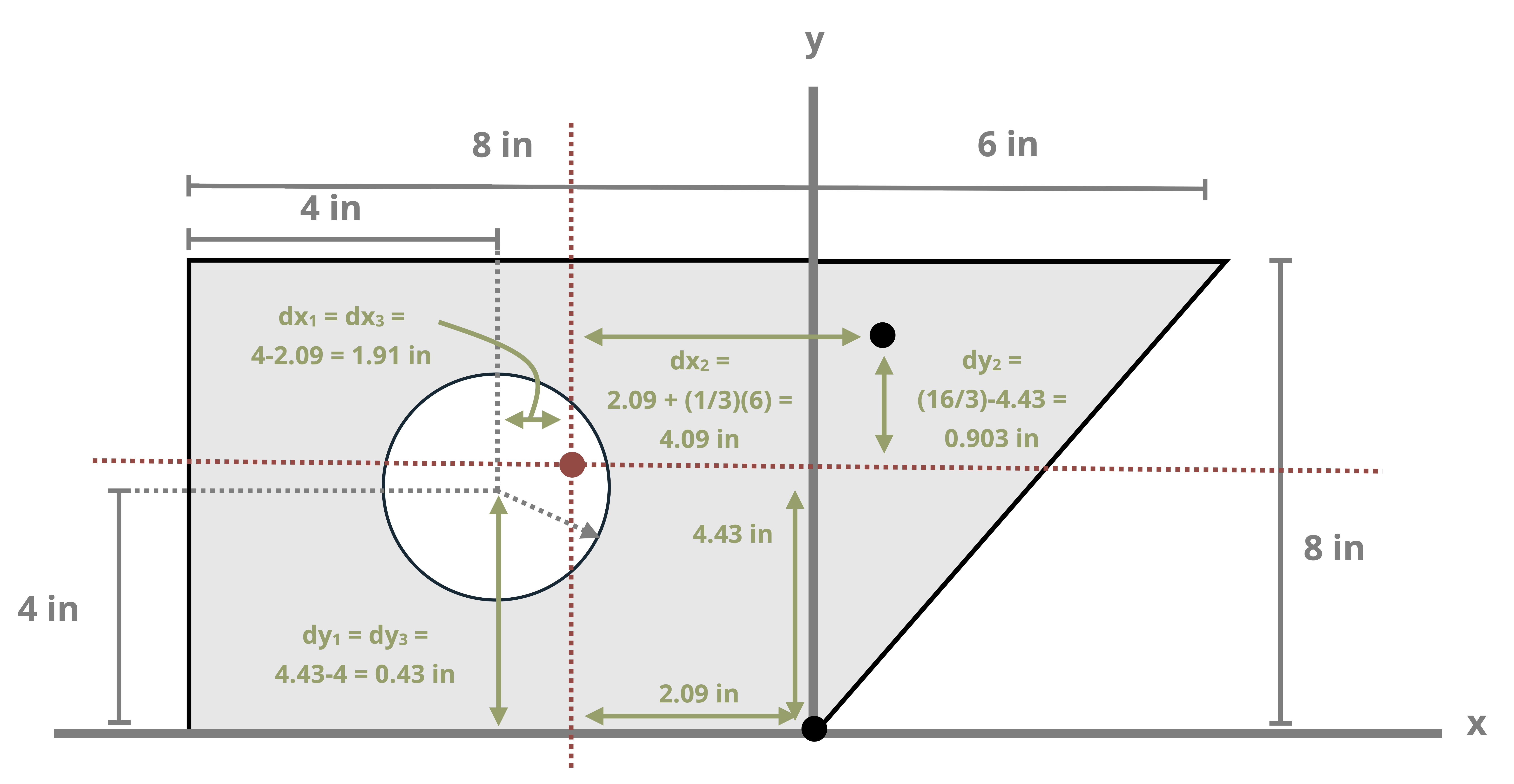
We found that the centroid is located 2.09 in. to the left of the y-axis and 4.43 in. up from the x-axis.
The next step is to break up the section into common shapes (see Appendix E) as shown in the following figure. Note that shape 3 is a hole, so we need to subtract the area and second moment of area.
The formula for the second moment of area of a shape are with respect to the shape’s centroid, not to the section’s overall centroid. Make a necessary adjustment using the parallel axis theorem to transform the rotational axis from the shape’s centroid to the section’s centroid. Do this for each shape.
Present this method in terms of a table, first for Ix then Iy.
| Shape | \(A{~(in.^2)}\) | \(I_x{~(in.^4)}\) | \(d_y{~(in.)}\) | \(I_x+Ad_y^2{~(in.^4)}\) |
|---|---|---|---|---|
| 1 | 64 | (1/12)(8)(8)3 = 341.3 |
0.43 | 341.3 + (64)(0.43)2 = 353.1 |
| 2 | 24 | (1/36)(6)(8)3 = 85.3 |
0.90 | 85.3 + (24)(0.9)2 = 104.7 |
| 3 | -4π | (-π/4)(2)4 = -12.6 |
0.43 | -12.6 + (-4π)(0.43)2 = -14.9 |
| Ix = 442.9 in.4 |
| Shape | \(A{~(in.^2)}\) | \(I_y{~(in.^4)}\) | \(d_x{~(in.)}\) | \(I_y+Ad_x^2{~(in.^4)}\) |
|---|---|---|---|---|
| 1 | 64 | (1/12)(8)(8)3 = 341.3 |
0.57 | 341.3 + (64)(0.57)2 = 362.1 |
| 2 | 24 | (1/36)(8)(6)3 = 48 |
1.43 | 48 + (24)(1.43)2 = 97.1 |
| 3 | -4π | (-π/4)(2)4 = -12.6 |
0.57 | -12.6 + (-4π)(0.57)2 = -16.7 |
| Iy = 442.5 in.4 |
The calculation and visualizations for each dx and dy term are as shown in the figure.
Summary
Click to expand
References
Click to expand
Figures
All figures in this chapter were created by Kindred Grey in 2025 and released under a CC BY license, except for
- Figure 8.1: Isometric view of concrete barriers used in roadway construction. Pushcreativity. 2008. CC BY-SA 3.0. https://commons.wikimedia.org/wiki/File:Concrete_step_barrier_3D_cross_section.jpg.